Reduced BCS Model

One-Sentence Description

The reduced BCS model is a finite set of doubly degenerate fermion levels with an all-to-all attraction that moves intact time-reversed pairs between levels, conserves particle number exactly, and admits Richardson’s exact fixed-number solution.

Canonical Scope

This dossier is the canonical home for:

• the finite-level, number-conserving reduced pairing Hamiltonian;
• active and Pauli-blocked pair orbitals;
• seniority sectors and their Hilbert-space dimensions;
• the Anderson pseudospin form of the exact model;
• Richardson’s product ansatz and coupled root equations;
• exact weak-, strong-, degenerate-shell, and one-pair limits;
• fixed-number pairing observables and parity effects;
• a direct-diagonalization benchmark for four levels and two pairs.

BCS Mean-Field Theory is the canonical derivation of the Cooper instability, anomalous decoupling, BCS state, gap and number equations, quasiparticles, and bulk thermodynamics. BCS Model is the compact lookup card. The present page instead keeps particle number sharp and treats the finite interacting Hamiltonian exactly.

That distinction is not cosmetic. The exact Hamiltonian satisfies

$$[H_{\mathrm{red}},\widehat N] = 0,$$

whereas its usual unprojected mean-field representative contains pair-creation and pair-annihilation terms. Broken $U(1)$ symmetry belongs to the thermodynamic mean-field description, not to literal number loss in the isolated finite model.

Why This Reduction Is Useful

A generic two-body interaction scatters fermions through many channels. The reduced model retains only zero-center-of-mass scattering between time-reversed pairs,

$$(i,\bar i) \longrightarrow (j,\bar j).$$

This reduction isolates three pieces of physics that are otherwise easy to conflate:

1. Pauli exclusion makes each pair orbital hard core.
2. An attractive interaction correlates many pair orbitals collectively.
3. A fixed-number finite system can have strong pairing correlations without a nonzero anomalous one-point function.

The model arose in nuclear pairing and later became central to the theory of ultrasmall superconducting grains, where the single-particle level spacing competes directly with the bulk pairing scale. It is also a clean example of an interacting integrable model: exact solvability reduces diagonalization to coupled nonlinear equations, but does not turn the Hamiltonian into a free theory.

Degrees of Freedom and Pair Orbitals

Let $i=1,\ldots,L$ label one-particle energies $\epsilon_i$. Each energy has two time-reversed fermion states, denoted $i$ and $\bar i$, with

$$\{c_i,c_j^\dagger\} = \delta_{ij}, \qquad \{c_i,c_{\bar j}^\dagger\} = 0.$$

Define an intact-pair operator by

$$b_i^\dagger = c_i^\dagger c_{\bar i}^\dagger, \qquad b_i = c_{\bar i}c_i.$$

The local Fock states are

$$\lvert0\rangle_i, \qquad c_i^\dagger\lvert0\rangle_i, \qquad c_{\bar i}^\dagger\lvert0\rangle_i, \qquad b_i^\dagger\lvert0\rangle_i.$$

Pair operators on distinct levels commute, but they are not canonical bosons:

$$[b_i,b_j^\dagger] = \delta_{ij} \left( 1-n_i-n_{\bar i} \right),$$

and

$$(b_i^\dagger)^2 = 0.$$

The nilpotency is the local Pauli constraint. A level can hold one intact pair, not an arbitrary boson occupation.

Hamiltonian and Conventions

The finite-level constant-pairing Hamiltonian used throughout this page is

$$\begin{aligned} H_{\mathrm{red}} ={}& \sum_{i=1}^{L} \epsilon_i \left( n_i+n_{\bar i} \right) \\ &- g \sum_{i,j=1}^{L} b_i^\dagger b_j, \qquad g\gt0. \end{aligned}$$

Thus $g\gt0$ means attraction. The interaction includes the diagonal terms $i=j$. Introducing

$$B^\dagger = \sum_{i=1}^{L}b_i^\dagger,$$

gives the compact form

$$H_{\mathrm{red}} = \sum_i \epsilon_i \left( n_i+n_{\bar i} \right) - gB^\dagger B.$$

The diagonal-term convention

Some authors restrict the interaction sum to $i\ne j$. In a sector with exactly $M$ intact pairs,

$$\sum_i b_i^\dagger b_i = M,$$

so omitting $i=j$ changes every energy in that sector by $+gM$ and leaves its eigenvectors unchanged. Richardson equations and quoted absolute energies must be compared only after this convention is aligned.

Canonical and grand Hamiltonians

The exact solution is most transparent for $H_{\mathrm{red}}$ at fixed particle number. A grand Hamiltonian is

$$K_{\mathrm{red}} = H_{\mathrm{red}} - \mu\widehat N.$$

Within a fixed-$N$ sector, this shifts every energy by $-\mu N$ without changing any eigenvector. Replacing $\epsilon_i$ by $\xi_i=\epsilon_i-\mu$ is therefore legitimate, but it should not be mistaken for changing the exact number symmetry.

Extensivity in a bulk limit

For a fixed finite shell, $g$ is simply an energy. In a thermodynamic sequence with mean level spacing $d\propto\mathcal V^{-1}$, one holds a dimensionless coupling such as

$$\lambda = \frac{g}{d}$$

fixed, or writes the interaction matrix element explicitly as a coupling divided by volume. Holding the finite-level matrix element $g$ fixed while sending the number of levels to infinity produces a different, generally superextensive scaling.

Blocking and Seniority

A singly occupied pair orbital cannot receive or emit an intact pair. Define the local seniority indicator

$$\widehat\nu_i = n_i+n_{\bar i} - 2n_in_{\bar i}.$$

Its eigenvalue is zero on empty and paired states and one on either singly occupied state. For the reduced Hamiltonian,

$$[H_{\mathrm{red}},\widehat\nu_i] = 0$$

for every level $i$. Hence every exact eigenproblem separates into:

• a blocked set $\mathcal B$ of singly occupied levels;
• an active set $\mathcal A$ of empty-or-paired levels;
• $M$ intact pairs on the active set;
• total particle number $N=2M+\nu$, where $\nu=|\mathcal B|$.

For a specified blocked set and specified orientations of its unpaired fermions, let

$$\Omega = |\mathcal A| = L-\nu.$$

The fixed-$M$ paired Hilbert-space dimension is

$$\dim\mathcal H_{\mathcal B,M} = \binom{\Omega}{M}.$$

The exact solver never needs to mix this sector with another particle number or blocked pattern. If spin orientations are also counted and the Hamiltonian has no spin-dependent term, each blocked set carries the expected orientation degeneracy.

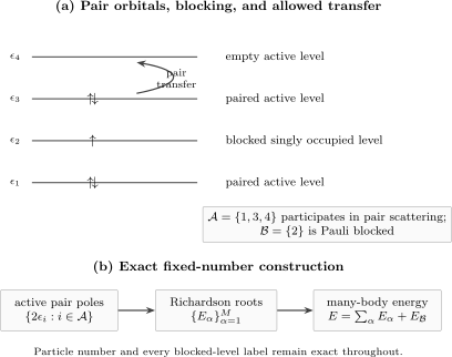
An intact pair can scatter between active levels while a singly occupied level is Pauli blocked. Richardson’s construction uses only the active pair poles $2\epsilon_i$; the blocked one-particle energy is added after the roots are summed.

Anderson Pseudospins

On each active level define

$$S_i^+ = b_i^\dagger, \qquad S_i^- = b_i,$$

and

$$S_i^z = \frac12 \left( n_i+n_{\bar i}-1 \right).$$

The empty and paired states form a pseudospin-$1/2$ doublet. On the active subspace,

$$[S_i^+,S_j^-] = 2\delta_{ij}S_i^z, \qquad [S_i^z,S_j^\pm] = \pm\delta_{ij}S_i^\pm.$$

The Hamiltonian in a fixed blocked sector is

$$\begin{aligned} H_{\mathcal B} ={}& E_{\mathcal B} + 2 \sum_{i\in\mathcal A} \epsilon_i \left( S_i^z+\frac12 \right) \\ &- g \sum_{i,j\in\mathcal A} S_i^+S_j^-, \end{aligned}$$

where

$$E_{\mathcal B} = \sum_{i\in\mathcal B}\epsilon_i.$$

The interaction is an all-to-all transverse ferromagnetic coupling in pseudospin language, while nondegenerate $\epsilon_i$ provide inhomogeneous longitudinal fields. Total

$$S^z = \sum_{i\in\mathcal A}S_i^z = M-\frac{\Omega}{2}$$

is fixed by pair number.

The pseudospins are an exact rewriting, not a semiclassical approximation. Replacing them by classical vectors or factorizing their correlations would be an additional mean-field step.

Symmetries and Conserved Data

Exact particle-number symmetry

Because each interaction term creates and annihilates one pair,

$$[\widehat N,b_i^\dagger b_j] = 0,$$

and therefore

$$[\widehat N,H_{\mathrm{red}}] = 0.$$

Fermion parity is consequently conserved as well, but it contains less information than the full $U(1)$ charge.

Level seniorities

Every $\widehat\nu_i$ is conserved. The reduced model cannot move an unpaired fermion between levels because it contains no one-body hopping term and no broken-pair scattering channel.

Time reversal

With real $g$, degenerate time-reversed partners, and no magnetic field, the Hamiltonian is time-reversal invariant. An odd number of fermions carries the corresponding Kramers structure when the microscopic particles have half-integer spin.

Permutations and collective spin

If several $\epsilon_i$ are equal, permutations within that degenerate shell are symmetries. When all active levels are degenerate, the Hamiltonian depends on collective pseudospin operators and total pseudospin $S$ is conserved. Generic nondegenerate levels break this collective $SU(2)$ symmetry while preserving integrability.

Richardson–Gaudin integrability

The constant-pairing Hamiltonian belongs to the rational Richardson–Gaudin family. It has a complete set of mutually commuting conserved operators for generic level data. Their existence explains why an interacting, nonuniform pseudospin model can be solved by Bethe-type spectral parameters. It does not imply ballistic transport, free quasiparticles, or solvability after arbitrary extra interactions are added.

Exact Solution Status

For a finite set of pairwise distinct levels and constant all-to-all pair coupling, the model is exactly solvable in every fixed blocked sector. Here “exact” means:

1. eigenvectors have a finite product form;
2. the product parameters satisfy explicitly known algebraic equations;
3. the many-body energy is an exact function of those parameters;
4. all states can be recovered by following the solution branches, with special treatment at singular parametrizations.

It does not mean that every root is available in elementary closed form. Solving many coupled Richardson equations can itself be numerically delicate.

The following changes generally leave the specific solution class:

• arbitrary nonseparable matrix elements $g_{ij}$;
• finite-center-of-mass pairing channels;
• pair-breaking interactions that mix seniorities;
• generic density, exchange, or spin-orbit terms;
• retarded interactions with independent frequency dynamics;
• coupling to an electromagnetic field beyond a specified integrable extension.

Some deformations belong to other Richardson–Gaudin families, but integrability must be demonstrated rather than inferred from the word “pairing.”

Richardson Product State

Choose a blocked reference state $\lvert\nu\rangle$ satisfying

$$b_i\lvert\nu\rangle = 0$$

for every active level. For each spectral parameter $E_\alpha$, define a collective pair operator

$$B_\alpha^\dagger = \sum_{i\in\mathcal A} \frac{S_i^+}{2\epsilon_i-E_\alpha}.$$

Richardson’s ansatz for $M$ pairs is

$$\lvert\Psi\rangle = \prod_{\alpha=1}^{M} B_\alpha^\dagger \lvert\nu\rangle.$$

The factors commute, but the roots do not label distinguishable physical pairs. Pauli exclusion couples all factors through the shared pseudospin operators.

Richardson equations

For the Hamiltonian and diagonal-term convention used here, the state is an eigenstate when

$$\frac1g - \sum_{i\in\mathcal A} \frac{1}{2\epsilon_i-E_\alpha} + \sum_{\substack{\beta=1\\\beta\ne\alpha}}^{M} \frac{2}{E_\beta-E_\alpha} = 0$$

for every $\alpha=1,\ldots,M$.

Once the equations hold, the exact many-body energy is

$$E = E_{\mathcal B} + \sum_{\alpha=1}^{M}E_\alpha.$$

The signs in the root equation depend on whether the pair operator is written with denominator $2\epsilon_i-E_\alpha$ or $E_\alpha-2\epsilon_i$, and quoted energies depend on whether diagonal interaction terms are included. A correct implementation states all three conventions together.

Why the equations appear

The one-body commutator is

$$\left[ 2\sum_i\epsilon_iS_i^z, B_\alpha^\dagger \right] = E_\alpha B_\alpha^\dagger + S^+,$$

where

$$S^+ = \sum_{i\in\mathcal A}S_i^+.$$

The interaction commutator produces the same unwanted vector $S^+$ multiplied by level-pole terms. Moving $S_i^z$ through the other collective pair factors adds the root–root terms. The residual coefficient of

$$S^+ \prod_{\beta\ne\alpha} B_\beta^\dagger \lvert\nu\rangle$$

is proportional to

$$1 - g \sum_{i\in\mathcal A} \frac{1}{2\epsilon_i-E_\alpha} + 2g \sum_{\beta\ne\alpha} \frac{1}{E_\beta-E_\alpha}.$$

Setting every residual to zero gives the Richardson equations. What looks like a root–root interaction is the algebraic trace of Pauli blocking among collective pairs.

Interpreting the Roots

One pair

For $M=1$, there is no root–root term and the equation becomes

$$\frac1g = \sum_{i\in\mathcal A} \frac{1}{2\epsilon_i-E}.$$

If the $2\epsilon_i$ are ordered and distinct, one solution lies below the lowest pair pole and one lies in every interval between neighboring poles. The lowest root is the collective attractive state.

More than one pair

For $M\gt1$, an individual $E_\alpha$ is a spectral parameter, not the energy of a separately observable molecule. The invariant energy is the sum of all roots. Permuting the roots does not create a new state.

For real $\epsilon_i$ and $g$, roots can be real or occur in complex-conjugate sets. The total energy remains real. A complex root is not a decay width and does not make the Hermitian Hamiltonian nonunitary.

Apparent singularities

During continuation in $g$, roots may approach a pole $2\epsilon_i$ or collide before leaving the real axis as a conjugate pair. The wavefunction can remain finite even when the chosen root coordinates are ill-conditioned. Stable solvers use continuation, symmetric root variables, eigenvalue-based variables, or other regularizations rather than interpreting every large intermediate term as a physical divergence.

Important Limits

Zero coupling

At $g=0$, eigenstates are occupation configurations. For a branch connected to occupied active levels $i_1,\ldots,i_M$,

$$E_\alpha \longrightarrow 2\epsilon_{i_\alpha}.$$

The roots begin at pair poles, which is precisely why direct Newton iteration at $g=0$ is singular. Numerical continuation starts at a small nonzero coupling.

Weak attraction

Let $\mathcal O$ be the $M$ occupied pair levels of a nondegenerate configuration and $\mathcal U$ the empty active levels. Ordinary perturbation theory gives

$$\begin{aligned} E ={}& 2\sum_{i\in\mathcal O}\epsilon_i -gM \\ &- g^2 \sum_{\substack{i\in\mathcal O\\a\in\mathcal U}} \frac{1}{2(\epsilon_a-\epsilon_i)} + O(g^3). \end{aligned}$$

The $-gM$ term comes from diagonal pair scattering. The second-order term comes from virtual transfer of one pair from an occupied to an empty level. Near degeneracies require degenerate perturbation theory instead.

Degenerate shell

Suppose all $\Omega$ active levels have energy $\epsilon_0$. Then

$$H = 2\epsilon_0M - gS^+S^-.$$

For total pseudospin $S$ and

$$m = M-\frac{\Omega}{2},$$

the energy is

$$E_{S,M} = 2\epsilon_0M - g \left[ S(S+1)-m(m-1) \right].$$

For attraction, the lowest state at fixed $M$ has maximal $S=\Omega/2$, so

$$E_0 = 2\epsilon_0M - gM(\Omega-M+1).$$

This result exposes the collective enhancement beyond the diagonal contribution $-gM$.

Strong attraction with nondegenerate levels

When $g$ exceeds the active-level bandwidth, the interaction first selects the maximal-pseudospin multiplet. Let

$$\bar\epsilon = \frac1\Omega \sum_{i\in\mathcal A}\epsilon_i.$$

The ground-state energy begins as

$$E_0 = -gM(\Omega-M+1) + 2M\bar\epsilon + O\!\left( \frac{W^2}{g} \right),$$

where $W$ is a scale for the level spread. The leading state is a number-projected collective pair state, not a product of localized level pairs.

One empty or one occupied pair orbital

At $M=0$ the active vacuum is exact. At $M=\Omega$, every active level is paired and off-diagonal transfer is Pauli blocked; the only interaction contribution is $-g\Omega$. These limits are useful checks because the nominally all-to-all interaction has no available destination for pair motion.

Relation to Bulk BCS Mean Field

The exact finite system and BCS mean field answer related but different questions.

Exact reduced model	BCS mean-field saddle
fixed $N$ can be imposed from the outset	usually grand canonical
quartic interacting Hamiltonian	self-consistent quadratic Hamiltonian
$\langle b_i\rangle=0$ in a number eigenstate	$\langle b_i\rangle$ can select a phase
Richardson roots encode finite-size correlations	gap and number equations encode the bulk saddle
seniority and parity effects are explicit	finite-size number fluctuations are usually suppressed only relatively

In an appropriate thermodynamic limit, the continuum distribution of Richardson roots reproduces the BCS gap and number conditions. This statement requires a declared level density, interaction scaling, filling, cutoff, and order of limits. It does not make the unprojected BCS wavefunction an exact finite-$L$ eigenstate.

For any fixed-number eigenstate,

$$\langle\Psi|b_i|\Psi\rangle = 0$$

because $b_i$ changes particle number by two. Pair coherence instead appears in the number-conserving matrix

$$C_{ij} = \langle\Psi| b_i^\dagger b_j |\Psi\rangle.$$

A large eigenvalue of $C$ is the fixed-number signature connected to pair condensation and off-diagonal long-range order. Off-Diagonal Long-Range Order owns the general criterion.

Typical Observables

Level occupations

The occupation of a time-reversed doublet is

$$N_i = \langle n_i+n_{\bar i}\rangle.$$

In an unblocked active level, $0\le N_i\le2$. A blocked level has $N_i=1$ exactly.

The Hellmann–Feynman theorem gives

$$N_i = \frac{\partial E}{\partial\epsilon_i}$$

when the derivative follows a nondegenerate eigenstate and the Hamiltonian convention is held fixed.

Collective pairing correlation

Because

$$\frac{\partial H}{\partial g} = -B^\dagger B,$$

one has

$$\langle B^\dagger B\rangle = -\frac{\partial E}{\partial g}.$$

This observable includes both the unavoidable diagonal pair count and coherent transfer terms. Reporting only $\langle B^\dagger B\rangle$ without subtracting or stating the diagonal baseline can overstate coherence.

Pair correlation matrix

The matrix

$$C_{ij} = \langle b_i^\dagger b_j\rangle$$

resolves where the collective correlation resides. Its trace is $M$ in a fixed-pair sector, while its largest eigenvalue measures collective concentration of pair weight.

Pair-breaking and parity energies

Breaking a pair changes seniority by two. A canonical pair-breaking gap compares the lowest energies in the relevant $\nu=0$ and $\nu=2$ sectors at fixed total particle number. Odd-even indicators compare neighboring ground-state energies, for example through a second difference such as

$$\Delta_P(N) = \frac{(-1)^N}{2} \left[ E_0(N+1)-2E_0(N)+E_0(N-1) \right],$$

with the sign convention stated explicitly. Charging energies and one-body offsets must be removed consistently before interpreting this as a pairing scale.

Response and matrix elements

Pair-addition, pair-removal, spin, and tunneling spectra require matrix elements between different Richardson states and often different seniority sectors. Exact energies alone do not determine spectral weights.

Physical Phenomena

Mesoscopic pairing

When the level spacing $d$ is not negligible relative to a bulk gap scale, finite particle number and discrete levels matter. The exact model tracks the smooth crossover from collective pairing to a fluctuation-dominated few-level regime without inventing a sharp finite-size phase transition.

Nuclear pairing

The same algebra describes idealized pairing among time-reversed nuclear orbitals. In realistic nuclei, shell degeneracies, angular-momentum coupling, proton-neutron channels, deformation, and additional residual interactions require extensions. The reduced model is a benchmark and organizing limit, not a complete nuclear Hamiltonian.

Parity and blocking

An odd fermion blocks one level and removes it from the coherent pair-scattering space. This changes correlation energies and excitation thresholds. The effect is kinematic as well as energetic: the active Richardson equations themselves use a different pole set.

Emergence of a broken-symmetry description

As the number of active levels grows with the proper extensive scaling, exact number-conserving correlations can support the thermodynamic phenomenology captured efficiently by a phase-selecting BCS saddle. The finite model therefore clarifies what spontaneous symmetry breaking summarizes rather than contradicting it.

Minimal Worked Example: Two Levels and One Pair

Take two levels

$$\epsilon_1 = -\frac d2, \qquad \epsilon_2 = \frac d2,$$

with $d\gt0$, one pair, and no blocked levels. In the basis

$$\lvert1\rangle = b_1^\dagger\lvert0\rangle, \qquad \lvert2\rangle = b_2^\dagger\lvert0\rangle,$$

the Hamiltonian is

$$H = \begin{pmatrix} -d-g & -g\\ -g & d-g \end{pmatrix}.$$

Its eigenvalues are

$$E_\pm = -g \pm \sqrt{d^2+g^2}.$$

The ground state may be written

$$\lvert\Psi_-\rangle = \cos\theta\,\lvert1\rangle + \sin\theta\,\lvert2\rangle,$$

where

$$\tan(2\theta) = \frac gd, \qquad 0\lt\theta\lt\frac\pi4.$$

At weak coupling the pair mostly occupies the lower level. At strong coupling $\theta\to\pi/4$ and the pair approaches an equal collective superposition.

The one-root Richardson equation is

$$\frac1g = \frac{1}{-d-E} + \frac{1}{d-E}.$$

Combining fractions gives

$$E^2 + 2gE - d^2 = 0,$$

which reproduces both exact eigenvalues. The collective pairing correlation in the ground state is

$$\langle B^\dagger B\rangle_- = 1 + \frac{g}{\sqrt{d^2+g^2}}.$$

The first term is the diagonal one-pair baseline; the second is coherent pair transfer.

Numerical Benchmark: Four Levels and Two Pairs

This benchmark tests direct diagonalization and Richardson roots independently. Use

$$\frac{\epsilon_i}{d} = \left( -\frac32, -\frac12, \frac12, \frac32 \right), \qquad \frac gd = \frac12,$$

with no blocked levels and $M=2$. Order the six basis states as

$$\left( \lvert12\rangle, \lvert13\rangle, \lvert14\rangle, \lvert23\rangle, \lvert24\rangle, \lvert34\rangle \right),$$

where

$$\lvert ij\rangle = b_i^\dagger b_j^\dagger\lvert0\rangle.$$

The dimension is

$$\binom42 = 6.$$

In the stated basis,

$$\frac Hd = \begin{pmatrix} -5 & -\tfrac12 & -\tfrac12 & -\tfrac12 & -\tfrac12 & 0\\ -\tfrac12 & -3 & -\tfrac12 & -\tfrac12 & 0 & -\tfrac12\\ -\tfrac12 & -\tfrac12 & -1 & 0 & -\tfrac12 & -\tfrac12\\ -\tfrac12 & -\tfrac12 & 0 & -1 & -\tfrac12 & -\tfrac12\\ -\tfrac12 & 0 & -\tfrac12 & -\tfrac12 & 1 & -\tfrac12\\ 0 & -\tfrac12 & -\tfrac12 & -\tfrac12 & -\tfrac12 & 3 \end{pmatrix}.$$

For $x=E/d$, the characteristic polynomial factors as

$$\det\!\left( xI-\frac Hd \right) = (x+1)^2 \left( x^4+4x^3-17x^2-40x+64 \right).$$

The ordered spectrum is

$$\begin{aligned} \frac{E_n}{d} = \{&-5.364451526424, -3.064618573309, -1, \\ &-1, 1.208940239171, 3.220129860562\}. \end{aligned}$$

For the ground-state branch, the Richardson roots are real at this coupling:

$$\frac{E_1}{d} = -3.380717508599, \qquad \frac{E_2}{d} = -1.983734017826.$$

Their sum gives

$$\frac{E_1+E_2}{d} = -5.364451526424,$$

in agreement with direct diagonalization.

Useful matrix invariants are

$$\operatorname{tr}\!\left( \frac Hd \right) = -6,$$ $$\operatorname{tr}\!\left[ \left( \frac Hd \right)^2 \right] = 52,$$

and

$$\det\!\left( \frac Hd \right) = 64.$$

For a normalized ground state with positive coefficients in the stated basis, the pair-level occupations are

$$\left( \langle b_i^\dagger b_i\rangle \right)_{i=1}^{4} = ( 0.96456324, 0.90142714, 0.09857286, 0.03543676 ),$$

and

$$\langle B^\dagger B\rangle = 3.54843564.$$

The occupation sum is exactly $M=2$. These values test eigenvector conventions in addition to the spectrum.

Benchmark contract

1. Generate the basis combinatorially; do not hard-code only the displayed matrix.
2. Verify Hermiticity and the three matrix invariants.
3. Reproduce the six eigenvalues and the double eigenvalue at $E/d=-1$.
4. Solve the two Richardson equations by continuation from small positive $g/d$.
5. Check each root residual and the sum-of-roots energy separately.
6. Verify that the pair occupations sum to two and that Hellmann–Feynman differentiation reproduces $\langle B^\dagger B\rangle$.

This finite exact problem is distinct from MB-B008, which tests a continuum mean-field self-consistency equation.

Numerical Strategy

Direct diagonalization

For a fixed blocked set, represent a basis state by an $\Omega$-bit string with $M$ occupied pair orbitals. The diagonal element is

$$H_{aa} = 2\sum_{i\in a}\epsilon_i - gM.$$

Two configurations have off-diagonal matrix element $-g$ if one is obtained from the other by moving exactly one pair from an occupied to an empty active level. Otherwise the matrix element vanishes.

Direct diagonalization scales with

$$\binom{\Omega}{M}$$

and is invaluable for small-system validation.

Richardson continuation

A practical root workflow is:

1. assign each branch to $M$ occupied pair poles at very small $g\gt0$;
2. solve at that coupling with high precision;
3. increase $g$ in adaptive steps using the previous roots as initial data;
4. preserve conjugate pairing for real Hamiltonian data;
5. monitor both equation residuals and the energy against independent invariants;
6. regularize near pole collisions rather than reducing precision blindly.

Newton convergence alone is not evidence that the desired eigenstate branch was followed. Different root solutions represent different many-body states.

Stable checks

At every coupling, verify:

$$\left| \frac1g - \sum_i\frac{1}{2\epsilon_i-E_\alpha} + \sum_{\beta\ne\alpha} \frac{2}{E_\beta-E_\alpha} \right| \lt \varepsilon_{\mathrm{root}},$$

the reality of the summed energy, continuity from the chosen $g\to0^+$ configuration, and agreement with exact diagonalization wherever the Hilbert space is small enough.

Variants and Boundaries of the Entry

Level degeneracy beyond one Kramers pair

Nuclear pairing often groups several magnetic substates into a level with pseudospin larger than $1/2$. Richardson equations then carry representation-dependent degeneracy or seniority weights. The spin-$1/2$ equations above apply to one doubly degenerate pair orbital per $i$.

Separable form factors

Interactions of the form

$$-g \sum_{i,j} w_iw_j b_i^\dagger b_j$$

motivate generalized pairing models. A separable appearance alone does not guarantee the same rational Richardson equations; the exact class depends on how level energies and form factors enter.

Number-projected BCS states

Projecting an unprojected BCS state onto fixed $N$ produces a useful variational state and restores exact charge. It is not generally identical to a finite-coupling Richardson eigenstate. Variational Many-Body States owns the broader variational context.

Pairing with finite center-of-mass momentum

Fulde–Ferrell–Larkin–Ovchinnikov-type channels and pair-density waves involve different pair labels and spatial structure. They are not contained in the zero-center-of-mass constant-pairing Hamiltonian by changing only a parameter.

Open and driven systems

Coupling the levels to particle reservoirs, losses, or time-dependent drives changes the symmetry and often the solution method. A non-Hermitian rapidity in such a model may carry decay information; a complex Richardson root in the closed Hermitian model does not.

Common Mistakes

• Saying that the exact reduced BCS Hamiltonian breaks particle-number symmetry.
• Calling the pair operators ordinary bosons and dropping their hard-core commutator.
• Leaving diagonal $i=j$ interaction terms unspecified when comparing energies.
• Treating a blocked singly occupied level as an active pole in the Richardson equations.
• Interpreting each root as a distinguishable, directly observable Cooper-pair energy.
• Treating complex-conjugate roots as complex many-body energies.
• Calling a numerical root solve “closed form,” or calling exact integrability “free.”
• Using the mean-field gap equation as an exact finite-size eigenvalue equation.
• Holding the finite-level matrix element $g$ fixed in a bulk limit without checking extensivity.
• Assuming arbitrary momentum-dependent pairing interactions retain Richardson–Gaudin integrability.
• Comparing number-projected and unprojected states without stating the ensemble and observable.
• Inferring a sharp finite-size phase transition from a smooth crossover or avoided crossing.

Summary

• The reduced BCS model moves intact time-reversed pairs between doubly degenerate levels.
• Its exact Hamiltonian conserves total particle number and every local seniority label.
• Singly occupied levels are Pauli blocked and are removed from the active root equations.
• Active empty and paired states form Anderson pseudospins.
• Richardson’s product state is exact when its $M$ roots satisfy $M$ coupled equations.
• The many-body energy is the sum of the roots plus blocked one-particle energies.
• Exact finite-size pairing and symmetry-breaking BCS mean field are complementary descriptions with different canonical observables.
• Direct diagonalization and root continuation should be cross-validated on small sectors.

Exercises

1. Number conservation and blocking

Show directly that

$$[\widehat N,b_i^\dagger b_j] = 0$$

and that $b_i^\dagger$ and $b_i$ both annihilate either singly occupied state on level $i$.

Solution

The number charges are

$$[\widehat N,b_i^\dagger] = 2b_i^\dagger, \qquad [\widehat N,b_j] = -2b_j.$$

Using the Leibniz rule,

$$\begin{aligned} [\widehat N,b_i^\dagger b_j] ={}& [\widehat N,b_i^\dagger]b_j + b_i^\dagger[\widehat N,b_j] \\ ={}& 2b_i^\dagger b_j - 2b_i^\dagger b_j = 0. \end{aligned}$$

For $c_i^\dagger\lvert0\rangle_i$, pair creation contains another $c_i^\dagger$ and vanishes by $(c_i^\dagger)^2=0$; pair annihilation finds no $\bar i$ fermion. The argument is identical with $i$ and $\bar i$ exchanged. Thus a singly occupied level is blocked.

2. One-pair root counting

Let $2\epsilon_1\lt\cdots\lt2\epsilon_\Omega$ and $g\gt0$. Show that the one-pair Richardson equation has one root below $2\epsilon_1$ and one root in every interval $(2\epsilon_i,2\epsilon_{i+1})$.

Solution

Define

$$f(E) = \frac1g - \sum_{i=1}^{\Omega} \frac{1}{2\epsilon_i-E}.$$

Away from poles,

$$f'(E) = -\sum_i \frac{1}{(2\epsilon_i-E)^2} \lt 0,$$

so $f$ is strictly decreasing on each interval. Below the first pole,

$$f(-\infty) = \frac1g \gt 0,$$

while $f(E)\to-\infty$ as $E\to(2\epsilon_1)^-$. There is exactly one root there. Immediately to the right of any pole $f\to+\infty$, and immediately to the left of the next pole $f\to-\infty$, giving exactly one root in each intervening interval. These $\Omega$ roots exhaust the one-pair Hilbert-space dimension.

3. Coherence in the two-level model

For the two-level one-pair ground state, derive the occupations of the lower and upper pair orbitals and check their strong-coupling limit.

Solution

With

$$\cos(2\theta) = \frac{d}{\sqrt{d^2+g^2}},$$

the pair occupations are

$$\langle b_1^\dagger b_1\rangle = \cos^2\theta = \frac12 \left( 1+ \frac{d}{\sqrt{d^2+g^2}} \right),$$

and

$$\langle b_2^\dagger b_2\rangle = \sin^2\theta = \frac12 \left( 1- \frac{d}{\sqrt{d^2+g^2}} \right).$$

They sum to one. As $g/d\to\infty$, both approach $1/2$, consistent with an equal collective superposition over the two levels.

4. Degenerate-shell ground energy

Derive

$$E_0 = 2\epsilon_0M - gM(\Omega-M+1)$$

for $M$ pairs in $\Omega$ degenerate active orbitals.

Solution

At fixed pair number,

$$m = M-\frac\Omega2.$$

The interaction is $-gS^+S^-$, and

$$S^+S^- = S(S+1)-S^z(S^z-1).$$

Attraction minimizes the energy by maximizing $S$, so $S=\Omega/2$. Therefore

$$\begin{aligned} S(S+1)-m(m-1) &= \left( \frac\Omega2+m \right) \left( \frac\Omega2-m+1 \right) \\ &= M(\Omega-M+1). \end{aligned}$$

Adding the one-body energy $2\epsilon_0M$ gives the result.

5. Matrix invariants in the four-level benchmark

Without diagonalizing the displayed $6\times6$ matrix, verify its trace and the trace of its square.

Solution

The diagonal entries are $-5,-3,-1,-1,1,3$, so

$$\operatorname{tr}(H/d) = -6.$$

For a real symmetric matrix,

$$\operatorname{tr}(A^2) = \sum_{a,b}|A_{ab}|^2.$$

The diagonal squares sum to

$$25+9+1+1+1+9 = 46.$$

There are twelve distinct undirected off-diagonal connections of magnitude $1/2$. Each appears twice in the double sum, so their contribution is

$$2\times12\times\frac14 = 6.$$

Hence

$$\operatorname{tr}[(H/d)^2] = 46+6 = 52.$$

6. Why the anomalous average vanishes

Let $\lvert\Psi_N\rangle$ be an exact number eigenstate. Prove that $\langle b_i\rangle=0$, and explain why this does not imply absent pairing correlations.

Solution

Since

$$\widehat N b_i\lvert\Psi_N\rangle = (N-2)b_i\lvert\Psi_N\rangle,$$

the vector $b_i\lvert\Psi_N\rangle$ lies in a particle-number sector orthogonal to $\lvert\Psi_N\rangle$. Therefore

$$\langle\Psi_N|b_i|\Psi_N\rangle = 0.$$

The neutral product $b_i^\dagger b_j$ preserves number, so

$$\langle\Psi_N|b_i^\dagger b_j|\Psi_N\rangle$$

can be nonzero. Pairing in a finite number-conserving system is diagnosed by this correlation matrix, pair-breaking energies, and related neutral observables rather than by a charge-two one-point function.

Cross-Links

• Model Encyclopedia Overview — comparison with lattice, impurity, gas, and frontier models.
• BCS Theory — bulk superconducting observables, weak-coupling scales, experimental inference, and the boundary to Eliashberg and unconventional regimes.
• BCS Mean-Field Theory — Cooper instability, gap equation, quasiparticles, and thermodynamics.
• BCS Model — compact model card.
• Fermionic Operators in Many-Body Models — Fock-space and anticommutation conventions.
• Number Operators and Conserved Quantities — exact charge bookkeeping versus number-breaking mean field.
• Bogoliubov Theory — fermionic quasiparticle transformations after mean-field decoupling.
• Variational Many-Body States — number-projected BCS and other ansatz families.
• Exact Solutions Preview — integrability and Bethe-ansatz context.
• Off-Diagonal Long-Range Order — number-conserving pair condensation criteria.
• Benchmark Problems — MB-B008, the separate mean-field gap-equation benchmark.
• Common Many-Body Hamiltonians — compact convention comparison.

References

1. R. W. Richardson, “A Restricted Class of Exact Eigenstates of the Pairing-Force Hamiltonian”, Physics Letters 3, 277–279 (1963) — original exact product construction.
2. R. W. Richardson and N. Sherman, “Exact Eigenstates of the Pairing-Force Hamiltonian”, Nuclear Physics 52, 221–238 (1964) — extended derivation and eigenstate structure.
3. R. W. Richardson, “Numerical Study of the 8–32-Particle Eigenstates of the Pairing Hamiltonian”, Physical Review 141, 949–956 (1966) — early exact numerical comparison with BCS theory.
4. J. Bardeen, L. N. Cooper, and J. R. Schrieffer, “Theory of Superconductivity”, Physical Review 108, 1175–1204 (1957) — canonical bulk mean-field theory and its microscopic setting.
5. J. von Delft and F. Braun, “Superconductivity in Ultrasmall Grains: Introduction to Richardson’s Exact Solution”, in Quantum Mesoscopic Phenomena and Mesoscopic Devices in Microelectronics (2000) — pedagogical finite-grain introduction.
6. G. Sierra, J. Dukelsky, G. G. Dussel, J. von Delft, and F. Braun, “Exact Study of the Effect of Level Statistics in Ultrasmall Superconducting Grains”, Physical Review B 61, R11890–R11893 (2000) — exact mesoscopic application.
7. J. von Delft and R. Poghossian, “Algebraic Bethe Ansatz for a Discrete-State BCS Pairing Model”, Physical Review B 66, 134502 (2002) — connection to commuting integrals and algebraic Bethe ansatz.
8. J. Dukelsky, S. Pittel, and G. Sierra, “Colloquium: Exactly Solvable Richardson–Gaudin Models for Many-Body Quantum Systems”, Reviews of Modern Physics 76, 643–662 (2004) — authoritative review of exact pairing models, electrostatic analogy, and the bulk BCS limit.
9. J. von Delft and D. C. Ralph, “Spectroscopy of Discrete Energy Levels in Ultrasmall Metallic Grains”, Physics Reports 345, 61–173 (2001) — experimental and theoretical context for level discreteness and parity effects.