Number Operators and Conserved Quantities

The total number operator counts the particles or quanta represented by a chosen set of modes:

$$\widehat N = \sum_i a_i^\dagger a_i.$$

Its many-body role is broader than counting. It generates a global $U(1)$ transformation, decomposes Fock space into fixed-number sectors, supplies selection rules, and gives a one-line test for whether a Hamiltonian preserves particle number:

$$[H,\widehat N] = 0.$$

The spectra and elementary ladder commutators are developed in Number Operators. This page is the many-body application guide: symmetry, charge counting, sector projectors, weighted conserved quantities, grand-canonical use, local versus global conservation, number-breaking mean field, fermion parity, and open-system sources.

Conventions

Unless stated otherwise:

• $a_i,a_i^\dagger$ denote bosonic or fermionic mode operators;
• $n_i=a_i^\dagger a_i$ is the occupation of complete mode $i$;
• $\widehat N=\sum_i n_i$ is the total number operator;
• $N$ without a hat is an eigenvalue of $\widehat N$;
• $\Pi_N$ projects onto the fixed-$N$ sector $\mathcal H_N$;
• $H$ acts on Fock space and is Hermitian;
• $M_{p,q}$ is a monomial with $p$ creation and $q$ annihilation operators;
• $U(\theta)=e^{-i\theta\widehat N}$ is the chosen global $U(1)$ convention.

With the opposite sign in the exponential, every phase below reverses. Conservation statements are unchanged.

Canonical Scope

This page owns the practical relation among:

• number operators and global $U(1)$ symmetry;
• charge counting of many-body operator strings;
• fixed-number blocks and selection rules;
• exact, explicit, spontaneous, and effective number breaking;
• exact reduced BCS pairing versus number-breaking BCS mean field;
• total number, local number, and reservoir exchange;
• numerical conservation checks.

Other pages retain their canonical roles:

• compact commutator, shift, parity, and bilinear formulas: Operator Identities;
• spectra and elementary ladder identities: Number Operators;
• operational superselection and reference frames: Particle-Number Superselection Preview;
• local densities, currents, and sources: Density Operators and Current Operators;
• general symmetry-conservation derivations: Commutators and Conservation Laws;
• grand-canonical weights and fluctuations: Grand-Canonical Ensemble.

Mode Number and Total Number

Each mode number is

$$n_i = a_i^\dagger a_i.$$

Its eigenvalue depends on statistics:

$$n_i \in \begin{cases} \{0,1,2,\ldots\},&\text{bosons},\\ \{0,1\},&\text{fermions}. \end{cases}$$

The total operator is the sum over the complete one-particle mode basis:

$$\widehat N = \sum_i n_i.$$

Individual $n_i$ depend on the chosen modes. The total $\widehat N$ does not change under a unitary rotation of the complete one-particle basis.

Total Number as a One-Body Lift

The identity on the one-particle Hilbert space lifts to total number:

$$\widehat N = d\Gamma(I_{\mathcal H_1}).$$

This explains several facts at once:

• $\widehat N$ is additive over particles;
• it has eigenvalue $N$ on the $N$-particle sector;
• it is basis independent;
• it is the natural generator of a common phase rotation of every mode.

The relation to general additive observables is developed in One-Body Operators.

Fock-Space Sector Decomposition

Bosonic or fermionic Fock space decomposes as

$$\mathcal F = \bigoplus_{N\in\mathcal S} \mathcal H_N,$$

where $\mathcal S=\{0,1,2,\ldots\}$ for an untruncated bosonic Fock space. For $M$ fermionic modes,

$$\mathcal S = \{0,1,\ldots,M\}.$$

The spectral resolution of total number is

$$\widehat N = \sum_{N\in\mathcal S} N\Pi_N,$$

with

$$\Pi_N\Pi_M = \delta_{NM}\Pi_N, \qquad \sum_N\Pi_N = I.$$

A vector can have components in several sectors even though the sectors are mutually orthogonal.

Number-Sector Projector

Because number eigenvalues are integers, the projector onto $\mathcal H_N$ has the Fourier representation

$$\Pi_N = \frac{1}{2\pi} \int_0^{2\pi} d\theta\, e^{i\theta(\widehat N-N)}.$$

Acting on a number eigenstate $\lvert M,\alpha\rangle$ gives

$$\Pi_N \lvert M,\alpha\rangle = \delta_{NM} \lvert M,\alpha\rangle.$$

This group-averaging formula is useful for number projection of variational states and for deriving sector-resolved partition functions.

Global U(1) Transformation

Define

$$U(\theta) = e^{-i\theta\widehat N}.$$

Using

$$[\widehat N,a_i] = -a_i, \qquad [\widehat N,a_i^\dagger] = a_i^\dagger,$$

one obtains

$$\begin{aligned} U(\theta)a_iU^\dagger(\theta) &= e^{i\theta}a_i, \\ U(\theta)a_i^\dagger U^\dagger(\theta) &= e^{-i\theta}a_i^\dagger. \end{aligned}$$

All modes receive the same phase. This is a global internal transformation, not a position-dependent gauge transformation.

Symmetry and Conservation

The Hamiltonian is invariant under this global $U(1)$ family when

$$U(\theta)HU^\dagger(\theta) = H$$

for every $\theta$. Differentiating at $\theta=0$ gives

$$[\widehat N,H] = 0.$$

Conversely, a vanishing commutator makes $H$ invariant under the generated unitary group. Thus, under the usual domain assumptions,

$$\text{global }U(1)\text{ invariance} \quad\Longleftrightarrow\quad [H,\widehat N]=0.$$

On a fixed-$N$ state, $U(\theta)$ produces only the ray phase $e^{-iN\theta}$. Across several number sectors it changes relative phases, and it acts nontrivially on charged operators.

Charge Counting for Operator Monomials

Let

$$M_{p,q} = a_{i_1}^\dagger\cdots a_{i_p}^\dagger a_{j_q}\cdots a_{j_1}.$$

Repeated use of the commutator product rule gives

$$[\widehat N,M_{p,q}] = (p-q)M_{p,q}.$$

The integer

$$r = p-q$$

is the number charge of the monomial: it maps the $N$ sector into the $N+r$ sector.

Equal numbers of creation and annihilation operators imply $r=0$. This term-by-term test is often faster and less error prone than constructing the full commutator matrix.

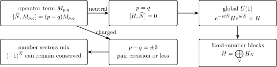
The difference $r=p-q$ between creation and annihilation counts is the number charge of a monomial. Neutral terms preserve every fixed-$N$ sector and the full global $U(1)$ symmetry. Terms with $r=\pm2$ mix number sectors but still preserve number parity.

Common Operator Charges

Term	Number charge	Consequence
$a_i^\dagger a_j$	$0$	transfers one particle; preserves total number
$a_i^\dagger a_j^\dagger a_l a_k$	$0$	pair scattering; preserves total number
$a_i^\dagger$	$+1$	creates one particle
$a_i$	$-1$	annihilates one particle
$a_i^\dagger a_j^\dagger$	$+2$	creates a pair
$a_j a_i$	$-2$	annihilates a pair
$a_i^\dagger a_j a_k$	$-1$	one creation and two annihilations

A Hermitian number-breaking Hamiltonian contains charge-changing terms in conjugate pairs. Hermiticity does not restore number conservation.

General Weighted Charges

Many conserved quantities are weighted mode occupations:

$$\widehat Q = \sum_i q_i n_i.$$

Then

$$[\widehat Q,a_i^\dagger] = q_i a_i^\dagger, \qquad [\widehat Q,a_i] = -q_i a_i.$$

For a monomial,

$$\begin{aligned} [\widehat Q,M_{p,q}] ={}& \left( \sum_{\alpha=1}^{p}q_{i_\alpha} - \sum_{\beta=1}^{q}q_{j_\beta} \right) M_{p,q}. \end{aligned}$$

This tests electric charge, species number, spin projection in an appropriate basis, or any Abelian additive quantum number. A process can violate the unweighted excitation count while conserving a physically weighted charge.

Number-Conserving Hamiltonians

A standard Hamiltonian with one- and two-body terms is

$$\begin{aligned} H ={}& \sum_{i,j} h_{ij}a_i^\dagger a_j \\ &+ \frac12 \sum_{i,j,k,l} V_{ij;kl} a_i^\dagger a_j^\dagger a_l a_k. \end{aligned}$$

Every monomial is neutral, so

$$[H,\widehat N] = 0.$$

The Hamiltonian may strongly mix mode occupations and generate correlations. Conservation of total number does not imply conservation of each $n_i$ or independent-particle dynamics.

Time-Dependent Hamiltonians

Explicit time dependence of $H(t)$ does not by itself break particle-number conservation. If

$$[H(t),\widehat N] = 0$$

for every time, then

$$\frac{d\widehat N_H}{dt} = \frac{i}{\hbar} [H_H(t),\widehat N_H] = 0.$$

A time-dependent hopping amplitude, trap, or interaction can preserve number. A coherent source or pair drive can break it. Energy conservation and number conservation are separate questions.

Block Diagonalization by Number

Insert fixed-number projectors around the commutator:

$$\Pi_N [\widehat N,H] \Pi_M = (N-M) \Pi_N H\Pi_M.$$

If $[\widehat N,H]=0$, then

$$\Pi_N H\Pi_M = 0 \qquad N\neq M.$$

Therefore

$$H = \bigoplus_N H_N, \qquad H_N = \Pi_N H\Pi_N.$$

Time evolution is block diagonal as well:

$$U(t,t_0) = \bigoplus_N U_N(t,t_0).$$

This is the algebraic reason fixed-number exact diagonalization is valid for a number-conserving Hamiltonian.

Conserved Number Distribution

For a state $\rho$, define

$$P_N = \operatorname{Tr}(\rho\Pi_N).$$

When $[H,\widehat N]=0$, every $P_N$ is constant under closed-system time evolution. Consequently, all moments

$$\langle\widehat N^m\rangle = \sum_N N^m P_N$$

are conserved.

This is stronger than conservation of the mean alone. A state can have constant $\langle\widehat N\rangle$ while its full number distribution changes under a specially engineered nonconserving process. Exact $U(1)$ symmetry freezes the entire distribution.

Conserved Does Not Mean Sharp

A number-conserving Hamiltonian does not force every state to have definite number. An initial state may contain several sectors:

$$\lvert\Psi(0)\rangle = \sum_N c_N\lvert\psi_N\rangle.$$

Each sector evolves independently:

$$\lvert\Psi(t)\rangle = \sum_N c_N U_N(t)\lvert\psi_N\rangle.$$

The probabilities $|c_N|^2$ are fixed, while relative sector phases and the internal states can evolve. Thus:

• conservation does not imply a sharp value;
• a sharp value does not by itself imply a superselection rule;
• an indefinite-number state does not by itself imply number-breaking dynamics.

Selection Rules from Number Charge

Suppose an operator $O_r$ satisfies

$$[\widehat N,O_r] = rO_r.$$

Between number eigenstates,

$$\begin{aligned} \langle N',\alpha'\vert [\widehat N,O_r] \vert N,\alpha\rangle ={}& (N'-N) \\ &\times \langle N',\alpha'\vert O_r \vert N,\alpha\rangle. \end{aligned}$$

Therefore a nonzero matrix element requires

$$N' = N+r.$$

In a fixed-number state, the expectation of every charged operator vanishes:

$$\langle O_r\rangle = 0 \qquad r\neq0.$$

This is why $\langle a_i\rangle$ and $\langle a_i a_j\rangle$ vanish in an exact number eigenstate even when one-body or pair coherence is physically strong.

Basis Invariance of Total Number

Let

$$b_\alpha = \sum_i U_{i\alpha}^*a_i$$

for unitary $U$. Then

$$\begin{aligned} \sum_\alpha b_\alpha^\dagger b_\alpha ={}& \sum_{i,j,\alpha} U_{i\alpha} U_{j\alpha}^* a_i^\dagger a_j \\ ={}& \sum_i a_i^\dagger a_i. \end{aligned}$$

Individual occupations transform into off-diagonal bilinears, but their complete sum remains $\widehat N$. A truncated or nonunitary change of one-particle space need not preserve this identity without a carefully transformed operator.

Species-Resolved Numbers

For several species or internal components,

$$\widehat N_s = \sum_i a_{is}^\dagger a_{is}, \qquad \widehat N = \sum_s \widehat N_s.$$

A Hamiltonian can conserve more than one number. Spin-conserving Hubbard hopping preserves $N_\uparrow$ and $N_\downarrow$ separately. A spin-flip term such as

$$H_{\mathrm{sf}} = \Omega \sum_i \left( c_{i\uparrow}^\dagger c_{i\downarrow} + c_{i\downarrow}^\dagger c_{i\uparrow} \right)$$

preserves $N_\uparrow+N_\downarrow$ but not the two component numbers separately.

The physically conserved combinations follow from all conversion terms, not from the labels chosen before writing the Hamiltonian.

Quasiparticle Number Is a Different Charge

Phonons, magnons, Bogoliubov modes, polaritons, and other quasiparticles have their own occupation operators. Their total occupation need not equal a microscopic particle number and is often not conserved.

A Hamiltonian diagonal in quasiparticle operators,

$$H_{\mathrm{qp}} = E_0 + \sum_\alpha E_\alpha \beta_\alpha^\dagger\beta_\alpha,$$

conserves $\sum_\alpha\beta_\alpha^\dagger\beta_\alpha$ only within that quadratic effective model. Interactions among quasiparticles can create and annihilate them while preserving an underlying atomic, electric, or spin charge.

Always name the counted degrees of freedom. Bogoliubov Quasiparticles works this distinction through explicitly for bosonic and fermionic transformations, including expected microscopic number, exact parity, and number-conserving formulations.

Local Number Versus Total Number

For a spatial region $\Omega$,

$$\widehat N_\Omega = \int_\Omega d^dr\, n(\mathbf r).$$

Even when total number is conserved, $\widehat N_\Omega$ generally is not. Particles can cross the boundary:

$$\frac{d\widehat N_\Omega}{dt} = - \int_{\partial\Omega} d\mathbf S\cdot \mathbf j_N + \widehat S_\Omega.$$

The source $\widehat S_\Omega$ vanishes for a locally number-conserving closed model. Taking $\Omega$ to be the complete closed system removes boundary flux and recovers global conservation.

The global commutator $[H,\widehat N]=0$ does not by itself identify a unique local current. Locality and the density decomposition are additional inputs.

Chemical Potential and the Grand Hamiltonian

When particle number is conserved, define

$$K = H-\mu\widehat N.$$

Then

$$[K,\widehat N] = 0.$$

On one fixed-$N$ sector,

$$K_N = H_N-\mu N I_N.$$

The chemical-potential term is a constant energy shift inside that sector. It does not change fixed-$N$ eigenvectors or closed-system expectation values. Its thermodynamic role is to change the relative weights assigned to different number sectors.

An equilibrium chemical potential normally couples to a conserved charge. If the proposed charge is not conserved by the microscopic isolated dynamics, the interpretation of its multiplier requires additional justification.

Grand-Canonical Mixtures Are Not Coherent Superpositions

For $[H,\widehat N]=0$, the grand-canonical density operator is block diagonal:

$$\rho_{\beta,\mu} = \bigoplus_N P_N\rho_{N,\beta}.$$

It is a statistical mixture over number sectors, not a coherent vector with an observable phase between sectors. Number fluctuations in this ensemble therefore do not by themselves violate a particle-number superselection restriction.

Conservation Is Not Superselection

Three statements must remain distinct:

1. $[H,\widehat N]=0$: the chosen closed-system dynamics preserves number sectors;
2. $\rho=\sum_N\Pi_N\rho\Pi_N$: the state has no inter-sector coherences;
3. $[A,\widehat N]=0$ for every allowed observable $A$: accessible operations cannot compare number-sector phases.

Only the third is an operational superselection restriction. A direct-sum decomposition or one commuting Hamiltonian is not enough to establish it. Reference frames, reservoirs, and enlarged descriptions can change which operations are available.

Fermion Parity

Define fermion parity spectrally by

$$P_F = (-1)^{\widehat N} = e^{i\pi\widehat N}.$$

It acts as

$$P_Fa_iP_F^\dagger = -a_i, \qquad P_Fa_i^\dagger P_F^\dagger = -a_i^\dagger.$$

An operator with even total ladder degree preserves fermion parity. In particular, pair creation and annihilation change $N$ by two, so they break continuous $U(1)$ number symmetry but preserve the discrete $\mathbb Z_2$ parity symmetry.

Bosonic models can also possess number parity when every process changes $N$ by an even integer. That model symmetry should not be conflated with the broader role of fermion parity in fermionic observable algebras.

Exact Reduced BCS Hamiltonian

Define the pair operators

$$b_{\mathbf k}^\dagger = c_{\mathbf k\uparrow}^\dagger c_{-\mathbf k\downarrow}^\dagger, \qquad b_{\mathbf k} = c_{-\mathbf k\downarrow} c_{\mathbf k\uparrow}.$$

A reduced BCS grand Hamiltonian is

$$\begin{aligned} K_{\mathrm{red}} ={}& \sum_{\mathbf k,\sigma} \xi_{\mathbf k} c_{\mathbf k\sigma}^\dagger c_{\mathbf k\sigma} \\ &- g \sum_{\mathbf k,\mathbf k'} b_{\mathbf k}^\dagger b_{\mathbf k'}, \end{aligned}$$

where $g>0$ denotes attraction in this convention. Since

$$[\widehat N,b_{\mathbf k}^\dagger] = 2b_{\mathbf k}^\dagger, \qquad [\widehat N,b_{\mathbf k}] = -2b_{\mathbf k},$$

the pair-scattering product is neutral:

$$[\widehat N,b_{\mathbf k}^\dagger b_{\mathbf k'}] = 0.$$

Therefore

$$[K_{\mathrm{red}},\widehat N] = 0.$$

The exact reduced pairing Hamiltonian scatters pairs; it does not create particles from nothing.

BCS Mean-Field Theory owns the full reduced-model, Cooper-instability, gap-equation, and quasiparticle derivation. The comparison here remains focused on number charge.

BCS Mean-Field Hamiltonian

Introduce

$$\Delta = g \sum_{\mathbf k} \langle b_{\mathbf k}\rangle.$$

The usual unprojected mean-field grand Hamiltonian has the form

$$\begin{aligned} K_{\mathrm{MF}} ={}& \sum_{\mathbf k,\sigma} \xi_{\mathbf k} c_{\mathbf k\sigma}^\dagger c_{\mathbf k\sigma} \\ &- \sum_{\mathbf k} \left( \Delta b_{\mathbf k}^\dagger + \Delta^*b_{\mathbf k} \right) + \frac{|\Delta|^2}{g}. \end{aligned}$$

Holding the chosen c-number $\Delta$ fixed,

$$\begin{aligned} [\widehat N,K_{\mathrm{MF}}] ={}& -2\sum_{\mathbf k} \Delta b_{\mathbf k}^\dagger \\ &+ 2\sum_{\mathbf k} \Delta^*b_{\mathbf k}, \end{aligned}$$

which is generally nonzero. The approximation mixes sectors whose particle numbers differ by two while preserving fermion parity.

This does not mean the underlying reduced BCS model violates particle-number conservation. The number breaking belongs to the symmetry-breaking mean-field representation. Reduced BCS Model develops the exact fixed-number sectors, blocking, and Richardson solution.

The thermodynamic saddle, coherence factors, and number-projected interpretation are developed in BCS Mean-Field Theory.

Phase of the Pair Field

Under the convention $U(\theta)=e^{-i\theta\widehat N}$,

$$b_{\mathbf k} \longmapsto e^{2i\theta}b_{\mathbf k}, \qquad \Delta \longmapsto e^{2i\theta}\Delta.$$

The family of mean-field Hamiltonians is covariant if $\Delta$ transforms with the anomalous average. Choosing one fixed phase for $\Delta$ selects a representative from that family.

In a finite exact number eigenstate,

$$\langle b_{\mathbf k}\rangle = 0$$

by the number selection rule. Pairing can instead appear in neutral quantities such as $\langle b_{\mathbf k}^\dagger b_{\mathbf k'}\rangle$. A source, phase reference, thermodynamic-limit construction, or number-projected state is needed to relate the exact and symmetry-breaking languages carefully.

Explicit, Spontaneous, and Effective Breaking

These phrases describe different physics.

Explicit breaking

The Hamiltonian itself does not commute with $\widehat N$. A coherent source is

$$H_{\mathrm{src}} = \sum_i \left( f_i a_i^\dagger + f_i^*a_i \right).$$

It changes subsystem number by one and fixes a phase reference.

Spontaneous breaking

The microscopic Hamiltonian preserves $U(1)$, but a thermodynamic-limit state or variational ansatz selects a phase. Finite-size exact eigenstates can remain number eigenstates even when neutral correlation functions reveal incipient order.

Effective breaking

The modeled subsystem exchanges particles with an omitted condensate, reservoir, drive, or reaction channel. The subsystem Hamiltonian or master equation need not conserve its number even when an enlarged closed description conserves a total charge.

Using the word “broken” without identifying which of these mechanisms is intended obscures the approximation.

Number-Changing Bosonic Terms

Bosonic effective models commonly contain a linear source or a pairing drive:

$$H_{\mathrm{pair}} = \frac12 \sum_{i,j} \left( \Delta_{ij}a_i^\dagger a_j^\dagger + \Delta_{ij}^*a_j a_i \right).$$

The source changes $N$ by one. The pair drive changes $N$ by two and can preserve bosonic number parity. Stability of a bosonic pairing Hamiltonian is a separate condition; a formal parity symmetry does not guarantee a spectrum bounded below.

A mean-field replacement $a_i\to\phi_i$ is an approximation involving a phase reference or symmetry-breaking limit. It is not an identity in a finite fixed-number Hilbert space.

Anomalous Expectations

An expectation such as

$$\langle a_i a_j\rangle$$

has number charge $-2$ in the commutator convention:

$$[\widehat N,a_i a_j] = -2a_i a_j.$$

It vanishes in a number eigenstate and in any $U(1)$-invariant density operator. A nonzero anomalous expectation therefore presupposes a number-breaking state description, a phase reference, or an enlarged relational interpretation.

Neutral pair correlations such as

$$\langle a_i^\dagger a_j^\dagger a_l a_k \rangle$$

can be nonzero without breaking number symmetry.

Open-System Number Balance

For a Lindblad–GKSL equation

$$\dot\rho = -\frac{i}{\hbar}[H,\rho] + \sum_\mu \kappa_\mu \mathcal D[L_\mu]\rho,$$

with

$$\mathcal D[L]\rho = L\rho L^\dagger - \frac12 \{L^\dagger L,\rho\},$$

the number expectation obeys

$$\begin{aligned} \frac{d}{dt} \langle\widehat N\rangle ={}& \frac{i}{\hbar} \langle[H,\widehat N]\rangle \\ &+ \sum_\mu \kappa_\mu \left\langle L_\mu^\dagger\widehat N L_\mu - \frac12 \{L_\mu^\dagger L_\mu,\widehat N\} \right\rangle. \end{aligned}$$

If

$$[\widehat N,L_\mu] = -r_\mu L_\mu$$

and $L_\mu^\dagger L_\mu$ commutes with $\widehat N$, that channel contributes

$$-r_\mu\kappa_\mu \langle L_\mu^\dagger L_\mu\rangle.$$

Single-particle loss has $r_\mu=1$, pair loss has $r_\mu=2$, and number dephasing with $L_\mu=n_i$ has $r_\mu=0$.

Numerical Conservation Tests

For a finite matrix representation, useful diagnostics are:

1. compute $C=[H,\widehat N]$ and compare $\lVert C\rVert$ with a scale such as $\lVert H\rVert\lVert\widehat N\rVert$;
2. inspect $\Pi_NH\Pi_M$ for $N\neq M$;
3. propagate states from one sector and monitor leakage;
4. monitor the full distribution $P_N$, not only $\langle\widehat N\rangle$;
5. test every weighted charge claimed by the model;
6. distinguish physical symmetry breaking from truncation or floating-point residuals;
7. verify that a basis transformation also transforms the charge operator;
8. test exact and mean-field Hamiltonians separately.

A numerical commutator should be judged relative to matrix scales and precision. Reporting only an absolute residual can be misleading.

Symmetry Reduction in Computation

When $[H,\widehat N]=0$, constructing only the required $N$ sector reduces memory and runtime. For $M$ modes,

$$\dim\mathcal H_N^{(F)} = \binom MN$$

for fermions, while for bosons

$$\dim\mathcal H_N^{(B)} = \binom{N+M-1}{N}.$$

Additional commuting charges can split the sector further. One must not impose a symmetry block that the actual Hamiltonian breaks; doing so silently removes physical matrix elements.

Common Mistakes

• Calling every mode occupation a conserved quantity.
• Assuming a time-dependent Hamiltonian necessarily breaks particle-number conservation.
• Checking only $\langle\widehat N\rangle$ instead of $[H,\widehat N]$ or the full distribution.
• Confusing a fixed-number state with a number-conserving Hamiltonian.
• Treating number conservation as an automatic superselection rule.
• Forgetting that $\widehat N$ is basis independent only under a complete unitary mode transformation.
• Claiming that exact reduced BCS pair scattering violates number conservation.
• Claiming that BCS mean field conserves $N$ because it preserves parity.
• Treating a nonzero anomalous average as compatible with an exact finite number eigenstate without a reference or projection argument.
• Confusing quasiparticle number with microscopic particle number.
• Adding $-\mu\widehat N$ to a fixed-$N$ problem and expecting eigenvectors to change.
• Inferring a local current from the global commutator alone.
• Interpreting subsystem loss as a fundamental violation when an omitted reservoir carries the compensating charge.
• Enforcing a symmetry sector numerically after adding a term that breaks it.

Quick Reference

Question	Diagnostic
Does a monomial conserve total number?	count $r=p-q$
Does the Hamiltonian have global $U(1)$ symmetry?	verify $[H,\widehat N]=0$
Which sectors can $O_r$ connect?	only $N\to N+r$
Is the Hamiltonian block diagonal?	check $\Pi_NH\Pi_M=0$ for $N\neq M$
Does pair creation preserve anything?	it breaks $U(1)$ but preserves number parity
Does a chemical potential alter fixed-$N$ eigenvectors?	no; $-\mu N$ is constant in that sector
Does a grand-canonical state require number coherence?	no; it is block diagonal when $[H,\widehat N]=0$
Does conservation imply superselection?	no; allowed operations must also be restricted
Is local number conserved?	derive its continuity equation and boundary flux
Does an open-system jump remove $r$ particles?	check $[\widehat N,L]=-rL$

Summary

• Total number is $d\Gamma(I_{\mathcal H_1})$ and is invariant under complete one-particle basis rotations.
• $\widehat N$ generates a global $U(1)$ transformation of the ladder operators.
• A monomial with $p$ creations and $q$ annihilations carries number charge $p-q$.
• $[H,\widehat N]=0$ makes the Hamiltonian and time evolution block diagonal in fixed-$N$ sectors.
• Number conservation preserves the full sector probability distribution, not merely its mean.
• Charged operators obey $N\to N+r$ selection rules and have zero expectation in fixed-number states.
• Separate species numbers survive only when conversion terms preserve them individually.
• Total conservation does not imply local conservation without a continuity equation.
• Exact reduced BCS pair scattering conserves $N$; unprojected BCS mean field breaks $U(1)$ but preserves fermion parity.
• Conservation, superselection, explicit breaking, spontaneous breaking, and open-system exchange are distinct statements.

Symmetry Sectors in Many-Body Numerics develops the computational use of fixed-$N$ and number-parity blocks, including dimension, closure, and sector-changing-observable checks.

Exercises

Exercise 1: Charge-counting theorem

Prove that a normally ordered monomial $M_{p,q}$ satisfies

$$[\widehat N,M_{p,q}] = (p-q)M_{p,q}.$$

Solution

Use

$$[\widehat N,a_i^\dagger] = a_i^\dagger, \qquad [\widehat N,a_i] = -a_i$$

and the product rule

$$[A,BC] = [A,B]C+B[A,C].$$

Each of the $p$ creation operators contributes $+M_{p,q}$ to the commutator, while each of the $q$ annihilation operators contributes $-M_{p,q}$. Summing the contributions gives

$$[\widehat N,M_{p,q}] = (p-q)M_{p,q}.$$

The result is the same for bosons and fermions because it uses ordinary commutators with the even operator $\widehat N$.

Exercise 2: Number selection rule

Let $[\widehat N,O_r]=rO_r$. Show that

$$\langle N',\alpha'\vert O_r \vert N,\alpha\rangle$$

vanishes unless $N'=N+r$.

Solution

Take the matrix element of the commutator:

$$\begin{aligned} \langle N',\alpha'\vert [\widehat N,O_r] \vert N,\alpha\rangle ={}& (N'-N) \\ &\times \langle N',\alpha'\vert O_r \vert N,\alpha\rangle. \end{aligned}$$

The defining relation gives the same left side as

$$r \langle N',\alpha'\vert O_r \vert N,\alpha\rangle.$$

Therefore

$$(N'-N-r) \langle N',\alpha'\vert O_r \vert N,\alpha\rangle = 0.$$

A nonzero matrix element requires $N'=N+r$.

Exercise 3: Basis invariance

For

$$b_\alpha = \sum_i U_{i\alpha}^*a_i,$$

with unitary $U$, prove

$$\sum_\alpha b_\alpha^\dagger b_\alpha = \sum_i a_i^\dagger a_i.$$

Solution

Substitute the mode transformation:

$$\begin{aligned} \sum_\alpha b_\alpha^\dagger b_\alpha ={}& \sum_{i,j,\alpha} U_{i\alpha} U_{j\alpha}^* a_i^\dagger a_j \\ ={}& \sum_{i,j} \delta_{ij} a_i^\dagger a_j \\ ={}& \sum_i a_i^\dagger a_i. \end{aligned}$$

Unitarity supplied

$$\sum_\alpha U_{i\alpha}U_{j\alpha}^* = \delta_{ij}.$$

The total is invariant, although each new $b_\alpha^\dagger b_\alpha$ is a linear combination of old diagonal and off-diagonal bilinears.

Exercise 4: Number blocks and sector probabilities

Assume $[H,\widehat N]=0$.

1. Show that $\Pi_NH\Pi_M=0$ for $N\neq M$.
2. Show that $P_N(t)=\operatorname{Tr}[\rho(t)\Pi_N]$ is constant under unitary evolution.

Solution

For the first part,

$$\Pi_N [\widehat N,H] \Pi_M = (N-M) \Pi_NH\Pi_M.$$

The left side vanishes. If $N\neq M$, division by $N-M$ gives

$$\Pi_NH\Pi_M = 0.$$

Thus $H$ commutes with every spectral projector $\Pi_N$. For the second part,

$$\begin{aligned} \frac{dP_N}{dt} &= -\frac{i}{\hbar} \operatorname{Tr} \left( [H,\rho]\Pi_N \right) \\ &= -\frac{i}{\hbar} \operatorname{Tr} \left( \rho[\Pi_N,H] \right) = 0. \end{aligned}$$

Every sector probability is conserved.

Exercise 5: Conversion between two species

Let

$$H_g = g \left( a^\dagger b + b^\dagger a \right).$$

Determine which of $N_a=a^\dagger a$, $N_b=b^\dagger b$, and $N_{\mathrm{tot}}=N_a+N_b$ are conserved.

Solution

The commutators are

$$\begin{aligned} [N_a,H_g] &= g \left( a^\dagger b - b^\dagger a \right), \\ [N_b,H_g] &= -g \left( a^\dagger b - b^\dagger a \right). \end{aligned}$$

Neither component number is conserved. Adding them gives

$$[N_{\mathrm{tot}},H_g] = 0.$$

The coupling converts one species into the other while preserving the total occupation.

Exercise 6: Exact and mean-field BCS number symmetry

Let $[\widehat N,b_{\mathbf k}^\dagger]=2b_{\mathbf k}^\dagger$ and $[\widehat N,b_{\mathbf k}]=-2b_{\mathbf k}$.

1. Show that $b_{\mathbf k}^\dagger b_{\mathbf k'}$ conserves number.
2. Show that $\Delta b_{\mathbf k}^\dagger+\Delta^*b_{\mathbf k}$ does not conserve number for fixed nonzero $\Delta$.
3. State which discrete symmetry remains.

Solution

For pair scattering,

$$\begin{aligned} [\widehat N, b_{\mathbf k}^\dagger b_{\mathbf k'}] ={}& 2b_{\mathbf k}^\dagger b_{\mathbf k'} - 2b_{\mathbf k}^\dagger b_{\mathbf k'} \\ ={}&0. \end{aligned}$$

For the mean-field pair source,

$$\begin{aligned} [\widehat N, \Delta b_{\mathbf k}^\dagger + \Delta^*b_{\mathbf k}] ={}& 2\Delta b_{\mathbf k}^\dagger \\ &- 2\Delta^*b_{\mathbf k}, \end{aligned}$$

which is generally nonzero. Both terms change particle number by an even integer, so fermion parity $(-1)^{\widehat N}$ remains conserved.

Exercise 7: Chemical potential in a fixed-number sector

Let $K=H-\mu\widehat N$ with $[H,\widehat N]=0$. Show that on $\mathcal H_N$, evolution under $K$ differs from evolution under $H$ only by a global phase.

Solution

On the fixed-$N$ sector,

$$K_N = H_N-\mu N I_N.$$

Because the second term is proportional to the identity,

$$\begin{aligned} e^{-iK_Nt/\hbar} &= e^{-i(H_N-\mu NI_N)t/\hbar} \\ &= e^{i\mu Nt/\hbar} e^{-iH_Nt/\hbar}. \end{aligned}$$

The prefactor is a global phase on $\mathcal H_N$, so every expectation value within that sector is unchanged. The chemical potential matters when comparing or statistically weighting different $N$ sectors.

Exercise 8: Single-particle loss

For one bosonic mode with number-conserving $H$ and master equation

$$\dot\rho = -\frac{i}{\hbar}[H,\rho] + \kappa\mathcal D[a]\rho,$$

derive the equation for $\langle n\rangle$.

Solution

The Hamiltonian contribution vanishes because $[H,n]=0$. For the dissipator, use

$$[n,a] = -a,$$

so the jump removes one quantum. The adjoint dissipator gives

$$\begin{aligned} \frac{d}{dt}\langle n\rangle ={}& \kappa \left\langle a^\dagger n a - \frac12 \{a^\dagger a,n\} \right\rangle \\ ={}& -\kappa \langle a^\dagger a\rangle. \end{aligned}$$

Therefore

$$\frac{d}{dt} \langle n\rangle = -\kappa\langle n\rangle,$$

with solution $\langle n(t)\rangle=e^{-\kappa t}\langle n(0)\rangle$. Number is not conserved in the subsystem because the environment receives the lost quanta.

References

1. A. L. Fetter and J. D. Walecka, Quantum Theory of Many-Particle Systems, Dover (2003).
2. J. W. Negele and H. Orland, Quantum Many-Particle Systems, Westview Press (1998).
3. P. Coleman, Introduction to Many-Body Physics, Cambridge University Press (2015).
4. A. Altland and B. Simons, Condensed Matter Field Theory, 2nd ed., Cambridge University Press (2010).
5. H. Bruus and K. Flensberg, Many-Body Quantum Theory in Condensed Matter Physics, Oxford University Press (2004).
6. L. Pitaevskii and S. Stringari, Bose–Einstein Condensation and Superfluidity, Oxford University Press (2016).
7. J. Bardeen, L. N. Cooper, and J. R. Schrieffer, “Theory of Superconductivity,” Physical Review 108, 1175–1204 (1957), doi:10.1103/PhysRev.108.1175.
8. G. C. Wick, A. S. Wightman, and E. P. Wigner, “The Intrinsic Parity of Elementary Particles,” Physical Review 88, 101–105 (1952), doi:10.1103/PhysRev.88.101.
9. Y. Aharonov and L. Susskind, “Charge Superselection Rule,” Physical Review 155, 1428–1431 (1967), doi:10.1103/PhysRev.155.1428.
10. S. D. Bartlett, T. Rudolph, and R. W. Spekkens, “Reference frames, superselection rules, and quantum information,” Reviews of Modern Physics 79, 555–609 (2007), doi:10.1103/RevModPhys.79.555.
11. G. Lindblad, “On the generators of quantum dynamical semigroups,” Communications in Mathematical Physics 48, 119–130 (1976), doi:10.1007/BF01608499.
12. V. Gorini, A. Kossakowski, and E. C. G. Sudarshan, “Completely positive dynamical semigroups of $N$-level systems,” Journal of Mathematical Physics 17, 821–825 (1976), doi:10.1063/1.522979.