Real-Space Representation

Real space makes spatial structure explicit. External potentials, interfaces, boundaries, disorder, local measurements, and short-range interactions appear where they act. A continuum field operator carries a position label; a lattice operator carries a site or localized-orbital label. Neither label is merely decorative: it determines which terms are local, which boundaries exist, and which approximations are controlled.

The continuum and lattice descriptions are related, but they are not interchangeable by typography alone. A trustworthy translation tracks the normalization of operators, the volume represented by each site, the scaling of couplings, the ultraviolet cutoff, and the boundary prescription.

This page develops that translation. The complementary Momentum-Space Representation explains how translation structure becomes mode-label algebra and momentum-conserving vertices.

Conventions

Unless stated otherwise:

• space has dimension $d$ and spatial domain $\Omega$;
• $\alpha,\beta$ label spin, species, orbital, or another internal component;
• $\psi_\alpha(\mathbf r)$ is a continuum annihilation field;
• $c_{j\alpha}$ annihilates a particle in a normalized cell or localized mode labeled by $j$;
• $a$ is a uniform lattice spacing and $a^d$ is the cell volume on a hypercubic grid;
• $\mathbf r_j$ is the position associated with site or cell $j$;
• $n(\mathbf r)=\sum_\alpha\psi_\alpha^\dagger(\mathbf r)\psi_\alpha(\mathbf r)$;
• $n_j=\sum_\alpha c_{j\alpha}^\dagger c_{j\alpha}$;
• upper signs in $[A,B]_{\mp}=AB\mp BA$ apply to bosons, and lower signs apply to fermions.

The symbol $c_j$ is used generically for a lattice mode. Statistics are fixed by its algebra, not by the letter.

Canonical Scope

This page owns:

• the many-body continuum Hamiltonian as a real-space representation;
• spatial locality of one-body and interaction terms;
• the normalized-cell dictionary between continuum fields and lattice operators;
• finite-difference kinetic energy and its small-spacing limit;
• scaling of densities and contact couplings under discretization;
• the distinction between lattice projection, spatial discretization, continuum limit, and thermodynamic limit;
• representation-level consequences of open, periodic, twisted, and wall boundary conditions;
• real-space validation and numerical cautions.

Other pages retain their canonical roles:

• field definitions, distributional algebra, and contact-interaction regularization: Field Operators in Many-Body Models;
• local densities, currents, and continuity equations: Density Operators and Current Operators;
• general matrix-element and reduced-density-matrix conventions: One-Body Operators and Two-Body Operators;
• self-adjoint operator domains and mathematical boundary theory: Domains of Operators and Boundary Conditions;
• model-family selection and chapter routing: Lattice Models and Spin Systems;
• model-specific hopping and phase structure: pages such as the Tight-Binding Model, Hubbard Model, Heisenberg Model, and XXZ Spin Chain.

Why Real Space Helps

Real space is often the natural representation when the problem contains:

• a trap, wall, interface, impurity, or spatially varying field;
• disorder that breaks translation symmetry;
• local interactions or measurements;
• finite samples and edge states;
• lattice geometry, coordination, or frustration;
• spatial correlation lengths, textures, or defects;
• local tensor-network or sparse-matrix structure.

Its cost is equally important. A translation-invariant kinetic term that is diagonal in momentum space becomes a differential operator or hopping matrix. Long-range interactions can connect many spatial points, and fermionic signs remain nonlocal in some tensor-product encodings even when the Hamiltonian is spatially local.

Continuum Field Coordinates

At equal time, continuum fields obey

$$[\psi_\alpha(\mathbf r), \psi_\beta^\dagger(\mathbf r')]_{\mp} = \delta_{\alpha\beta} \delta^{(d)}(\mathbf r-\mathbf r'),$$

with the same-statistics annihilation-annihilation and creation-creation brackets equal to zero.

The position label does not turn $\psi(\mathbf r)$ into an ordinary oscillator at each mathematical point. The field is an operator-valued distribution. Controlled operators are obtained by smearing it against normalized functions,

$$c_f = \int_\Omega d^dr\, f^*(\mathbf r) \psi(\mathbf r),$$

where

$$\int_\Omega d^dr\, |f(\mathbf r)|^2 = 1.$$

Then

$$[c_f,c_g^\dagger]_{\mp} = \langle f|g\rangle.$$

The foundational meaning of these expressions is developed in Field Operators. Here they are the starting point for spatial Hamiltonians and controlled discretizations.

Dimensions and Normalization

Because $\delta^{(d)}(\mathbf r)$ has dimensions $L^{-d}$, the field has engineering dimension

$$[\psi] = L^{-d/2}.$$

Consequently,

$$[n(\mathbf r)] = L^{-d},$$

and the total number operator is dimensionless:

$$\widehat N = \int_\Omega d^dr\, n(\mathbf r).$$

A lattice annihilation operator $c_j$ and occupation $n_j$ are dimensionless. Any continuum-to-lattice rule must supply the missing cell-volume factors.

General Real-Space Hamiltonian

A broad number-conserving continuum Hamiltonian is

$$\begin{aligned} H = {}& \sum_{\alpha,\beta} \int_\Omega d^dr\,d^dr'\, \psi_\alpha^\dagger(\mathbf r) h_{\alpha\beta}(\mathbf r,\mathbf r') \psi_\beta(\mathbf r') \\ &+ \frac12 \sum_{\alpha,\beta} \int_\Omega d^dr\,d^dr'\, \psi_\alpha^\dagger(\mathbf r) \psi_\beta^\dagger(\mathbf r') \\ &\qquad\times v_{\alpha\beta}(\mathbf r,\mathbf r') \psi_\beta(\mathbf r') \psi_\alpha(\mathbf r). \end{aligned}$$

The first line is one-body even when its kernel is spatially nonlocal. The remaining lines are two-body because they act on particle pairs. Spatial locality and particle rank are different classifications.

Hermiticity requires

$$h_{\alpha\beta}(\mathbf r,\mathbf r') = h_{\beta\alpha}^*(\mathbf r',\mathbf r),$$

together with the appropriate exchange and Hermiticity properties of $v_{\alpha\beta}$.

Local One-Body Terms

For nonrelativistic particles without internal mixing, a standard local one-particle operator is

$$h_0 = -\frac{\hbar^2}{2m}\nabla^2 + U(\mathbf r).$$

Its many-body lift is

$$H_0 = \int_\Omega d^dr\, \psi^\dagger(\mathbf r) \left[ -\frac{\hbar^2}{2m}\nabla^2 + U(\mathbf r) \right] \psi(\mathbf r).$$

The potential term is multiplicative and point-local. The kinetic term is local as a differential operator: it couples arbitrarily nearby field values through derivatives, but it does not contain an independent integral over a distant point.

Internal components allow a local matrix,

$$H_0 = \sum_{\alpha,\beta} \int_\Omega d^dr\, \psi_\alpha^\dagger(\mathbf r) [h_0(\mathbf r)]_{\alpha\beta} \psi_\beta(\mathbf r).$$

Zeeman terms, local species conversion, and some spin-orbit couplings fit this structure, although derivative spin-orbit terms require the same domain and boundary care as kinetic energy.

Kinetic Energy and Surface Terms

Integration by parts gives

$$\begin{aligned} \int_\Omega d^dr\, \psi^\dagger(-\nabla^2)\psi = {}& \int_\Omega d^dr\, \nabla\psi^\dagger \boldsymbol\cdot \nabla\psi \\ &- \int_{\partial\Omega}dS\, \psi^\dagger\partial_n\psi, \end{aligned}$$

where $\partial_n$ is the outward normal derivative. Therefore

$$T = \frac{\hbar^2}{2m} \int_\Omega d^dr\, |\nabla\psi|^2$$

is equivalent to the $-\nabla^2$ form only when the boundary contribution vanishes or is included separately.

This is not a cosmetic issue. Boundary data are part of the Hamiltonian domain, and changing them can change spectra, conserved currents, and edge physics.

External Potentials, Traps, and Disorder

A scalar external potential contributes

$$H_U = \int_\Omega d^dr\, U(\mathbf r)n(\mathbf r).$$

Examples include:

• a harmonic trap $U(\mathbf r)=m\omega^2r^2/2$;
• a wall or barrier;
• a periodic optical or crystalline potential;
• a random potential $U_\omega(\mathbf r)$ for one disorder realization;
• a slowly varying probe coupled to density.

Disorder averages do not replace sample-level quantum expectation values. A calculation should distinguish $\langle\cdot\rangle$ in a fixed realization from a later ensemble average over $\omega$.

Nonlocal Pair Interactions

For a translation-invariant, spin-independent pair potential,

$$\begin{aligned} H_{\mathrm{int}} = {}& \frac12 \int_\Omega d^dr\,d^dr'\, \psi^\dagger(\mathbf r) \psi^\dagger(\mathbf r') \\ &\times v(\mathbf r-\mathbf r') \psi(\mathbf r') \psi(\mathbf r). \end{aligned}$$

The factor $1/2$ prevents double counting unordered pairs. The kernel can be short-ranged without being point-local. Coulomb, dipolar, screened, and finite-range model interactions retain a genuine two-position structure.

In density language, one often writes schematically

$$H_{\mathrm{int}} = \frac12 \int d^dr\,d^dr'\, v(\mathbf r-\mathbf r') {:}n(\mathbf r)n(\mathbf r'){:}_0,$$

where the vacuum normal ordering removes a self-contraction. Coincident points and singular kernels still require a regulator or physical matching prescription.

Local Contact Interactions

For spinless bosons, the standard zero-range effective operator is

$$H_{\mathrm c}^{(B)} = \frac g2 \int_\Omega d^dr\, \psi^\dagger \psi^\dagger \psi \psi.$$

All fields are evaluated at the same position. Since $[\psi]=L^{-d/2}$, the coupling has units

$$[g] = \text{energy}\times L^d.$$

For two fermionic components, a common contact term is

$$H_{\mathrm c}^{(F)} = g \int_\Omega d^dr\, \psi_\uparrow^\dagger \psi_\downarrow^\dagger \psi_\downarrow \psi_\uparrow.$$

There is no displayed factor $1/2$ because the expression counts one pair of distinct components. A same-component point $s$-wave term vanishes formally for fermions, but finite-range and higher-partial-wave interactions remain possible.

These formulas define effective operators, not regulator-independent bare products at a point. Field Operators in Many-Body Models owns the scattering-length and ultraviolet cautions.

Local Densities and Regions

The number in a spatial region $A\subset\Omega$ is

$$N_A = \int_A d^dr\, n(\mathbf r).$$

Unlike total number, $N_A$ generally changes because particles cross the boundary $\partial A$. Its Heisenberg derivative is controlled by boundary flux and any local source terms. The canonical derivation belongs to Density Operators and Current Operators.

Local observables are often distributions too. A detector has a finite response profile $f_A(\mathbf r)$, leading to a smeared observable

$$N[f_A] = \int d^dr\, f_A(\mathbf r)n(\mathbf r).$$

This finite resolution is physically meaningful and becomes essential when comparing continuum formulas with lattice cells or numerical grids.

Correlation Functions in Real Space

The equal-time one-body density matrix is

$$G_{\alpha\beta}^{(1)} (\mathbf r,\mathbf r') = \left\langle \psi_\alpha^\dagger(\mathbf r) \psi_\beta(\mathbf r') \right\rangle.$$

Its diagonal gives density. Off-diagonal decay diagnoses coherence, but it is basis- and gauge-covariant rather than a standalone local observable.

A connected density correlator is

$$C_n(\mathbf r,\mathbf r') = \langle n(\mathbf r)n(\mathbf r')\rangle - \langle n(\mathbf r)\rangle \langle n(\mathbf r')\rangle.$$

At coincident points, operator ordering and contact terms matter. Cell-integrated or normal-ordered quantities are often safer than an unqualified value at $\mathbf r=\mathbf r'$.

Normalized Cell Modes

Partition space into disjoint cells $C_j$ of volume $\Delta V_j$. A normalized top-hat cell function is

$$w_j(\mathbf r) = \begin{cases} (\Delta V_j)^{-1/2}, &\mathbf r\in C_j,\\ 0,&\mathbf r\notin C_j. \end{cases}$$

Define

$$c_{j\alpha} = \int_\Omega d^dr\, w_j^*(\mathbf r) \psi_\alpha(\mathbf r).$$

Disjoint normalized cells satisfy

$$[c_{i\alpha},c_{j\beta}^\dagger]_{\mp} = \delta_{ij}\delta_{\alpha\beta}.$$

If the field varies slowly within a cell, midpoint quadrature gives

$$c_{j\alpha} \simeq \sqrt{\Delta V_j}\, \psi_\alpha(\mathbf r_j).$$

Equivalently,

$$\psi_\alpha(\mathbf r_j) \simeq \frac{c_{j\alpha}} {\sqrt{\Delta V_j}}.$$

This relation is the normalization core of the continuum–lattice dictionary.

Uniform-Grid Dictionary

For a hypercubic grid with cell volume $a^d$,

$$c_{j\alpha} \simeq a^{d/2} \psi_\alpha(\mathbf r_j),$$

and

$$\delta^{(d)} (\mathbf r_i-\mathbf r_j) \longleftrightarrow \frac{\delta_{ij}}{a^d}.$$

The associated quadrature rule is

$$\int_\Omega d^dr\, f(\mathbf r) \simeq a^d \sum_j f(\mathbf r_j).$$

Combining these rules gives

$$\int d^dr\, \psi^\dagger\psi \simeq \sum_j c_j^\dagger c_j.$$

No extra factor of $a^d$ remains in total number because the two field operators contribute $a^{-d}$.

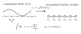
A real-space lattice operator represents a normalized cell mode, not the value of a dimensionless field at a point. In one dimension, $c_j\simeq\sqrt a\,\psi(x_j)$; in $d$ dimensions, $\sqrt a$ becomes $a^{d/2}$.

Density and Occupation

The site occupation approximates the number in one cell:

$$n_j = c_j^\dagger c_j \simeq a^d n(\mathbf r_j).$$

Thus a continuum density is not numerically equal to a site occupation. Their dimensions differ. At fixed physical density $n$, the mean occupation of an increasingly small cell scales as

$$\langle n_j\rangle \sim a^d n \longrightarrow 0$$

as $a\to0$.

For distinct cells,

$$\langle n_i n_j\rangle_{\mathrm c} \simeq a^{2d} C_n(\mathbf r_i,\mathbf r_j).$$

At the same cell, the exact comparison involves a double cell integral and operator-ordering contact terms rather than simple point sampling.

Localized Orbitals Beyond Top-Hat Cells

A physical lattice model often uses localized orbitals $w_{j\alpha}(\mathbf r)$ rather than grid cells:

$$c_{j\alpha} = \int d^dr\, w_{j\alpha}^*(\mathbf r) \psi(\mathbf r).$$

If the retained orbitals are orthonormal, the $c_{j\alpha}$ obey canonical mode algebra. The projected field is

$$\psi(\mathbf r) \approx \sum_{j,\alpha} w_{j\alpha}(\mathbf r) c_{j\alpha}.$$

The approximation sign records omitted orbitals or bands. Unlike top-hat discretization, neighboring localized orbitals can overlap spatially while remaining orthogonal through sign and phase structure.

A site can therefore mean a cell, atomic orbital, Wannier orbital, quantum dot, trap minimum, or graph vertex. The physical meaning must be stated.

Projected One-Body Matrix

Projecting a continuum one-particle operator gives

$$h_{i\alpha,j\beta} = \int d^dr\, w_{i\alpha}^*(\mathbf r) h_0 w_{j\beta}(\mathbf r),$$

and

$$H_0 = \sum_{i,j} \sum_{\alpha,\beta} h_{i\alpha,j\beta} c_{i\alpha}^\dagger c_{j\beta}.$$

Diagonal entries are onsite energies. Off-diagonal entries transfer particles between localized modes and are called hopping or hybridization amplitudes.

Spatially local $h_0$ does not imply a strictly nearest-neighbor projected matrix. Exponentially localized orbitals often produce exponentially decaying longer-range hopping, which is then truncated only with an accuracy criterion.

Projected Interactions

A continuum pair interaction projects to

$$\begin{aligned} V_{i\alpha,j\beta;k\gamma,l\delta} = {}& \int d^dr\,d^dr'\, w_{i\alpha}^*(\mathbf r) w_{j\beta}^*(\mathbf r') \\ &\times v(\mathbf r,\mathbf r') w_{k\gamma}(\mathbf r) w_{l\delta}(\mathbf r'). \end{aligned}$$

Keeping only onsite density interactions is an additional approximation. Projection can generate nearest-neighbor repulsion, exchange, pair hopping, density-assisted hopping, and longer-range terms even when a simple model later discards them.

For a contact interaction and a single localized orbital per equivalent site, the leading onsite coefficient is

$$U = g \int d^dr\, |w_j(\mathbf r)|^4.$$

This physical-orbital formula differs conceptually from the grid-regulator rule $U=g/a^d$, although a top-hat cell reproduces the latter.

Generic Lattice Hamiltonian

A common real-space lattice Hamiltonian is

$$\begin{aligned} H = {}& \sum_{i,j} \sum_{\alpha,\beta} h_{i\alpha,j\beta} c_{i\alpha}^\dagger c_{j\beta} \\ &+ \frac12 \sum_{i,j} V_{ij} {:}n_i n_j{:}_0 + H_{\mathrm{other}}. \end{aligned}$$

The first term includes onsite energies and hopping. The second displays a density interaction, while $H_{\mathrm{other}}$ may contain exchange, pair hopping, spin couplings, pairing, or higher-body operators. Lattice Models Overview develops the general model-building roles of these terms and their site, link, and plaquette supports.

The coefficient matrix must satisfy

$$h_{i\alpha,j\beta} = h_{j\beta,i\alpha}^*.$$

For an oriented hopping convention,

$$H_t = -\sum_{\langle i,j\rangle} \left( t_{ij}c_i^\dagger c_j + t_{ij}^*c_j^\dagger c_i \right),$$

which is manifestly Hermitian when each unoriented bond is counted once.

Onsite Interactions

For one bosonic mode per site,

$$H_U^{(B)} = \frac U2 \sum_j n_j(n_j-1).$$

The factor $n_j(n_j-1)/2$ counts unordered onsite pairs. Replacing it by $n_j^2/2$ adds a one-body term $Un_j/2$.

For spin-$1/2$ fermions,

$$H_U^{(F)} = U \sum_j n_{j\uparrow}n_{j\downarrow}.$$

Two opposite-spin modes can occupy the same site. A same-mode onsite pair vanishes by the fermionic algebra.

These operators are local in the chosen site basis. Whether that basis is sharply localized in physical space depends on how the lattice model was derived.

Spatial Locality on a Lattice

On a geometric lattice or graph, locality is measured by graph distance. A finite-range Hamiltonian can be written

$$H = \sum_X h_X,$$

where each $h_X$ acts only on a bounded cluster $X$ and its norm and range obey stated bounds.

Nearest-neighbor does not mean weak. It means that the operator support is restricted to adjacent sites. Conversely, a one-body hopping term can be long-ranged while remaining one-body.

The graph itself is part of the model. Coordination number, loops, dimensionality, boundary vertices, and sublattices affect spectra and correlations even when every bond carries the same coefficient.

Discretizing the Kinetic Energy

On a uniform hypercubic grid, a positive nearest-neighbor discretization is

$$T_a = t \sum_{j,\mu} \left( c_{j+\widehat\mu}^\dagger-c_j^\dagger \right) \left( c_{j+\widehat\mu}-c_j \right),$$

with

$$t = \frac{\hbar^2}{2ma^2}.$$

For periodic boundaries, expanding the squares gives

$$\begin{aligned} T_a = {}& -t \sum_{j,\mu} \left( c_j^\dagger c_{j+\widehat\mu} + c_{j+\widehat\mu}^\dagger c_j \right) \\ &+ 2dt \sum_j n_j. \end{aligned}$$

The onsite shift $2dt$ is part of this discretized Laplacian. Dropping it changes the zero of one-particle energy. At fixed total number a uniform shift can be harmless, but in grand-canonical calculations it shifts the chemical potential.

Small-Momentum Check

The periodic-grid dispersion is

$$\varepsilon_a(\mathbf k) = 2t \sum_{\mu=1}^d \left[ 1-\cos(k_\mu a) \right].$$

For $|k_\mu a|\ll1$,

$$1-\cos(k_\mu a) = \frac{k_\mu^2a^2}{2} + O(k_\mu^4a^4),$$

so

$$\varepsilon_a(\mathbf k) = \frac{\hbar^2k^2}{2m} + O\!\left( \frac{\hbar^2a^2k^4}{m} \right).$$

This is a low-momentum statement. The full lattice band is bounded and periodic in reciprocal space, unlike the unbounded quadratic continuum dispersion.

Boundary Sites in the Discrete Laplacian

For an open graph, the link-square kinetic term becomes

$$T_a = t \sum_{\langle i,j\rangle} (c_i^\dagger-c_j^\dagger) (c_i-c_j).$$

Its onsite coefficient is $t z_i$, where $z_i$ is the degree of site $i$. Boundary sites have smaller $z_i$ than bulk sites.

This operator has a uniform zero mode on a connected graph and resembles a Neumann-type discretization. A Dirichlet wall is not obtained merely by deleting wraparound bonds. One must specify endpoint placement, fixed boundary values, ghost cells, or equivalent boundary onsite terms.

The phrase open boundary therefore needs a precise matrix definition when a lattice is intended to approximate a continuum differential operator.

Discretizing a Scalar Potential

Using $n_j\simeq a^d n(\mathbf r_j)$,

$$\int d^dr\, U(\mathbf r)n(\mathbf r) \simeq \sum_j U(\mathbf r_j)n_j.$$

The onsite coefficient is the sampled potential energy; it does not acquire an additional $a^d$ factor.

For a cell average, a more accurate coefficient is

$$U_j = \int_{C_j}d^dr\, |w_j(\mathbf r)|^2 U(\mathbf r).$$

Midpoint sampling is controlled only when $U$ and the retained fields vary slowly on the cell scale.

Contact Coupling on a Grid

The bosonic contact term discretizes as

$$\begin{aligned} \frac g2 \int d^dr\, \psi^{\dagger2}\psi^2 &\simeq \frac g{2a^d} \sum_j c_j^{\dagger2}c_j^2 \\ &= \frac U2 \sum_j n_j(n_j-1), \end{aligned}$$

with

$$U = \frac g{a^d}.$$

The same cell-volume scaling applies to a two-component fermionic contact interaction. The divergence of the bare lattice coefficient as $a\to0$ is not by itself a physical divergence; a point coupling carries inverse-volume normalization on the grid.

In dimensions where contact physics requires renormalization, holding a naive $g$ fixed is generally insufficient. The cutoff-dependent lattice coupling must be matched to a physical scattering observable.

Nonlocal Interaction on a Grid

For separated cells, a density interaction discretizes as

$$\begin{aligned} H_V \simeq \frac12 \sum_{i,j} v(\mathbf r_i,\mathbf r_j) {:}n_i n_j{:}_0. \end{aligned}$$

There is no extra $a^{2d}$ because each continuum density contributes $a^{-d}$ while the two integration measures contribute $a^{2d}$.

Singular kernels, coincident cells, and long-range periodic sums need additional prescriptions. For Coulomb interactions, neutrality, boundary conditions, and treatment of the zero mode are part of the model.

Projection Is Not Discretization

Two constructions can produce similar-looking lattice operators:

1. Basis projection: retain selected localized orbitals of a physical continuum problem. The lattice spacing and orbital shape are physical model data, and omitted bands produce projection error.
2. Spatial discretization: replace a continuum field by cells or grid values as a numerical regulator. The spacing is intended to decrease, and finite-difference error is monitored as $a\to0$.

The coefficient $U=g\int|w_j|^4$ belongs to a general orbital projection. The special rule $U=g/a^d$ follows from top-hat grid cells. Conflating the two can produce incorrect scaling and false continuum claims.

What a Continuum Limit Requires

A continuum limit sends

$$a\longrightarrow0$$

while physical lengths, densities, masses, and renormalized observables are controlled. It is not simply the replacement of a sum by an integral.

One must specify:

• which low-energy modes are retained;
• how hopping and interaction coefficients scale with $a$;
• which physical quantities are held fixed;
• how the ultraviolet cutoff is removed or matched;
• how lattice anisotropy and irrelevant operators vanish;
• which boundary condition survives the limit.

Near a single quadratic band minimum $\mathbf k_0$, a slowly varying envelope can require

$$c_j \sim a^{d/2} e^{i\mathbf k_0\cdot\mathbf r_j} \psi(\mathbf r_j).$$

Several inequivalent minima can produce several continuum fields. A naive single-field limit would then discard valley or flavor structure.

Continuum and Thermodynamic Limits Differ

The continuum limit controls resolution:

$$a\to0 \quad\text{at controlled physical size}.$$

The thermodynamic limit controls volume:

$$L_{\mathrm{phys}}\to\infty \quad\text{at controlled density}.$$

A calculation may need both, but they answer different questions and need not commute. Thermodynamic Limit owns the general limit-order analysis.

At fixed physical size, decreasing $a$ increases the number of sites. At fixed $a$, increasing the number of sites changes the physical volume. Reporting only the site count leaves these operations ambiguous.

Ultraviolet and Infrared Scales

A spatial grid introduces a momentum scale of order

$$\Lambda_{\mathrm{UV}} \sim \frac{\pi}{a}.$$

A finite periodic box of linear size $L$ has momentum spacing

$$\Delta k = \frac{2\pi}{L}.$$

Thus $a$ controls ultraviolet resolution while $L$ controls infrared resolution. Reliable calculations vary them separately.

A hypercubic grid also reduces continuous rotational symmetry to the lattice point group. At low momentum the leading quadratic dispersion becomes isotropic, while higher-order corrections retain lattice anisotropy.

Boundary Conditions Define the Representation

The differential expression $-\nabla^2$ does not define a unique Hamiltonian without a spatial domain and operator domain. Typical continuum conditions include:

$$\psi|_{\partial\Omega}=0 \qquad \text{Dirichlet},$$ $$\partial_n\psi|_{\partial\Omega}=0 \qquad \text{Neumann},$$

and

$$\partial_n\psi = \kappa\psi \qquad \text{Robin},$$

with a suitable real boundary parameter $\kappa$ in the simplest scalar case.

Periodic or twisted conditions identify opposite faces:

$$\psi(\mathbf r+L_\mu\widehat\mu) = e^{i\theta_\mu} \psi(\mathbf r).$$

These choices change the allowed modes and can change finite-size observables even when the bulk differential expression is unchanged.

Hermiticity Boundary Form

For one-particle test functions $\phi$ and $\chi$,

$$\begin{aligned} &\langle\phi,-\nabla^2\chi\rangle - \langle-\nabla^2\phi,\chi\rangle \\ &= \int_{\partial\Omega}dS\, \left[ (\partial_n\phi^*)\chi - \phi^*\partial_n\chi \right]. \end{aligned}$$

A valid self-adjoint domain makes the appropriate boundary form vanish for every pair of domain functions and also satisfies maximality conditions. Dirichlet, Neumann, periodic, and suitable Robin conditions do so in standard settings.

The many-body field expansion must use one-particle modes belonging to the chosen domain. Boundary conditions are therefore built into the real-space field representation through its mode basis.

Open, Periodic, and Twisted Lattices

For a finite lattice:

• open boundaries omit couplings beyond the edge;
• periodic boundaries add bonds identifying opposite edges;
• twisted boundaries attach a phase to boundary crossing or distribute the same total phase over bulk bonds by a gauge transformation.

In one dimension, a boundary hopping can be written

$$H_{\partial} = -t \left( e^{i\theta}c_{L-1}^\dagger c_0 + e^{-i\theta}c_0^\dagger c_{L-1} \right).$$

The phase $\theta$ is gauge invariant modulo $2\pi$ as the total flux or twist around the ring, although its placement on individual bonds is gauge dependent.

Detailed fermion-parity and finite-size-sector cautions belong to the dedicated lattice-boundary treatment later in the volume. Here the essential point is that the hopping matrix itself must encode the boundary choice.

Boundaries Break Translation Symmetry

An open finite sample generally lacks exact translation symmetry. Momentum need not label eigenstates, even if every bulk bond has the same coefficient.

Periodic boundaries restore a discrete translation group when all coefficients respect the identification. Twisted boundaries can retain translation symmetry after the phase is distributed uniformly, but the allowed crystal momenta are shifted.

Boundary effects are often localized near an edge only in gapped systems with a finite correlation length and away from protected boundary modes. Near criticality or with long-range interactions, finite boundaries can influence the whole sample.

Real-Space Gauge Coupling

In a continuum electromagnetic field, kinetic momentum uses

$$-i\hbar\nabla \longrightarrow -i\hbar\nabla-q\mathbf A(\mathbf r).$$

On a lattice, gauge covariance is represented by link phases,

$$t_{ij} \longrightarrow t_{ij} \exp\!\left[ \frac{iq}{\hbar} \int_{\mathbf r_j}^{\mathbf r_i} \mathbf A\boldsymbol\cdot d\boldsymbol\ell \right].$$

The phase assigned to one link depends on gauge, while the phase around a closed loop measures flux and is gauge invariant. This bridge is developed physically in the Peierls Phase Preview.

Real-Space Matrix Structure

A local lattice Hamiltonian is usually sparse in the occupation-number basis. Each hopping term changes occupations on a small set of sites, and onsite interactions are diagonal in the site-occupation basis.

This structure favors:

• sparse exact diagonalization on small systems;
• matrix-product-state methods in one dimension;
• real-space quantum Monte Carlo in sign-compatible models;
• finite-difference or finite-element discretizations for continuum fields;
• local update and domain-decomposition strategies.

Sparsity does not remove exponential Hilbert-space growth. Bosons still need occupation cutoffs in finite computations, and fermions require a sign-consistent mode ordering.

Locality and Entanglement Structure

Ground states of many gapped short-range Hamiltonians have spatially organized entanglement, which is one reason local tensor-network descriptions can work well. This is not a universal guarantee. Critical states, Fermi surfaces, long-range interactions, highly excited states, and real-time evolution can require rapidly growing resources.

A basis change can hide spatial locality. A Hamiltonian sparse in site labels can become dense in momentum labels, while a diagonal free Hamiltonian in momentum space becomes hopping in real space. The physics is unchanged only when the transformation and any truncation are handled consistently.

Observables Under Discretization

For a uniform cell grid,

$$\langle c_{i\alpha}^\dagger c_{j\beta}\rangle \simeq a^d G_{\alpha\beta}^{(1)} (\mathbf r_i,\mathbf r_j).$$

A region occupation is approximated by

$$N_A \simeq \sum_{j:\,C_j\subset A} n_j,$$

with partial-cell weights needed near a curved or moving boundary.

Derivatives require a matching discrete operator. It is inconsistent to evolve with one lattice Laplacian and evaluate kinetic energy or current using an unrelated stencil without quantifying the difference.

Improving a Spatial Discretization

The nearest-neighbor Laplacian has errors of order $a^2$ for smooth fields. Accuracy can be improved by:

• higher-order finite-difference stencils;
• finite elements adapted to geometry;
• spectral bases for smooth periodic problems;
• nonuniform grids near sharp features;
• improved lattice operators that cancel leading anisotropic corrections.

Improvement often extends the hopping range. A more accurate real-space derivative can therefore be less local on the grid while better approximating a local continuum operator.

Every refinement should preserve Hermiticity, the intended boundary condition, and any exact symmetry that the discretization is meant to retain.

When Real Space Is the Wrong Basis

Real space may be inefficient when:

• the system is exactly translation invariant and kinetic energy dominates;
• conserved momentum sectors provide a large block reduction;
• the desired observable is naturally spectral;
• a long-range kernel is diagonal or nearly diagonal after Fourier transformation;
• the state occupies only a small set of delocalized modes.

Mixed representations can be optimal. Examples include real space in confined directions and momentum space along periodic directions, or localized orbitals for interactions and band eigenstates for propagation.

Reliable Construction Workflow

1. State whether the spatial labels are continuum points, numerical cells, physical orbitals, or abstract graph sites.
2. Declare particle statistics, internal components, and field normalization.
3. Specify the domain, geometry, and boundary conditions.
4. Write one-body and interaction kernels before imposing range truncations.
5. If projecting, define and normalize the retained orbitals.
6. If discretizing, write the quadrature and discrete derivative explicitly.
7. Track every factor of cell volume in fields, densities, and contact couplings.
8. Separate the continuum limit from the thermodynamic limit.
9. Check Hermiticity, particle-number conservation, and boundary flux.
10. Repeat calculations at finer spacing or in a larger basis to establish convergence.

Validation Checks

Useful algebraic checks include

$$[c_{i\alpha},c_{j\beta}^\dagger]_{\mp} = \delta_{ij}\delta_{\alpha\beta},$$ $$\widehat N \simeq \sum_j n_j,$$

and

$$h_{i\alpha,j\beta} = h_{j\beta,i\alpha}^*.$$

For a kinetic discretization, also test:

• nonnegative one-particle eigenvalues after the chosen energy shift;
• the expected small-$k$ quadratic dispersion;
• convergence under $a\to a/2$ at fixed physical size;
• the intended boundary zero modes or wall behavior;
• recovery of total-number conservation;
• agreement between link-square and matrix forms.

Common Mistakes

• Treating $\psi(\mathbf r_j)$ as a dimensionless lattice annihilation operator.
• Forgetting $c_j\simeq a^{d/2}\psi(\mathbf r_j)$.
• Equating site occupation with continuum density instead of cell-integrated number.
• Calling a one-body nonlocal kernel a two-body interaction.
• Assuming a local continuum operator projects to strictly nearest-neighbor hopping.
• Confusing a physical orbital projection with a regulator grid.
• Dropping the onsite shift in a discrete Laplacian without tracking the energy or chemical-potential change.
• Assuming that deleting a periodic bond automatically implements a continuum Dirichlet wall.
• Holding a bare contact coefficient fixed while changing the ultraviolet cutoff without matching.
• Taking a continuum limit by increasing the number of sites at fixed spacing.
• Taking a thermodynamic limit by decreasing spacing at fixed physical size.
• Ignoring cell averages for singular potentials or coincident correlators.
• Treating boundary conditions as an afterthought rather than part of the Hamiltonian.
• Assuming spatial locality removes fermionic sign or many-body complexity.

Quick Reference

Continuum quantity	Uniform-grid counterpart
$\psi(\mathbf r_j)$	$c_j/a^{d/2}$
$\delta^{(d)}(\mathbf r_i-\mathbf r_j)$	$\delta_{ij}/a^d$
$\int d^dr$	$a^d\sum_j$
$n(\mathbf r_j)$	$n_j/a^d$
$\int U n$	$\sum_j U_j n_j$
$-\hbar^2\nabla^2/(2m)$	link hopping with $t=\hbar^2/(2ma^2)$
contact coupling $g$	onsite $U=g/a^d$ for top-hat cells
ultraviolet scale	$\Lambda_{\mathrm{UV}}\sim\pi/a$
finite physical size $L$	infrared spacing $\Delta k\sim2\pi/L$

Summary

Real-space representation exposes where operators act. In the continuum, fields carry dimension $L^{-d/2}$ and Hamiltonians are written as spatial integrals of local or nonlocal kernels. On a lattice, normalized mode operators are dimensionless, locality is defined by site or graph support, and boundaries are encoded directly in the coefficient matrices.

The central dictionary is

$$c_j \simeq a^{d/2}\psi(\mathbf r_j), \qquad n_j \simeq a^d n(\mathbf r_j).$$

It determines the scaling of number, potential energy, kinetic hopping, and contact interactions. A continuum limit additionally requires parameter matching, cutoff control, and a declared boundary prescription. A lattice projection, a numerical discretization, and a thermodynamic limit are distinct operations even when their Hamiltonians look similar.

Exercises

Exercise 1: Canonical algebra of cell modes

For disjoint cells $C_i$ with normalized top-hat functions $w_i$, prove that

$$[c_{i\alpha},c_{j\beta}^\dagger]_{\mp} = \delta_{ij}\delta_{\alpha\beta}.$$

Solution

By definition,

$$c_{i\alpha} = \int d^dr\, w_i^*(\mathbf r) \psi_\alpha(\mathbf r).$$

Therefore

$$\begin{aligned} [c_{i\alpha},c_{j\beta}^\dagger]_{\mp} = {}& \int d^dr\,d^dr'\, w_i^*(\mathbf r) w_j(\mathbf r') \\ &\times [\psi_\alpha(\mathbf r), \psi_\beta^\dagger(\mathbf r')]_{\mp}. \end{aligned}$$

Insert the field algebra:

$$\begin{aligned} [c_{i\alpha},c_{j\beta}^\dagger]_{\mp} &= \delta_{\alpha\beta} \int d^dr\, w_i^*(\mathbf r)w_j(\mathbf r) \\ &= \delta_{\alpha\beta} \langle w_i|w_j\rangle. \end{aligned}$$

Disjoint normalized top-hat functions are orthonormal, so $\langle w_i|w_j\rangle=\delta_{ij}$.

Exercise 2: Number and density scaling

Use $c_j\simeq a^{d/2}\psi(\mathbf r_j)$ to derive the lattice approximation to total number and the relation between $\langle n_j\rangle$ and continuum density.

Solution

The local occupation is

$$n_j = c_j^\dagger c_j \simeq a^d \psi^\dagger(\mathbf r_j) \psi(\mathbf r_j) = a^d n(\mathbf r_j).$$

Summing over cells gives

$$\sum_j n_j \simeq a^d \sum_j n(\mathbf r_j) \simeq \int d^dr\, n(\mathbf r) = \widehat N.$$

Taking an expectation value yields

$$\langle n_j\rangle \simeq a^d \langle n(\mathbf r_j)\rangle.$$

The site occupation is a cell-integrated number, while the continuum density is number per volume.

Exercise 3: Expand the link-square kinetic energy

For a one-dimensional periodic chain, expand

$$T_a = t\sum_j (c_{j+1}^\dagger-c_j^\dagger) (c_{j+1}-c_j)$$

and identify the hopping and onsite terms.

Solution

Expanding one link gives

$$\begin{aligned} (c_{j+1}^\dagger-c_j^\dagger) (c_{j+1}-c_j) = {}& n_{j+1}+n_j \\ &-c_{j+1}^\dagger c_j -c_j^\dagger c_{j+1}. \end{aligned}$$

With periodic boundaries, every site appears in two neighboring links. Hence

$$T_a = -t\sum_j \left( c_j^\dagger c_{j+1} + c_{j+1}^\dagger c_j \right) + 2t\sum_j n_j.$$

The second term fixes the bottom of the discrete Laplacian spectrum at zero.

Exercise 4: Recover the continuum dispersion

Show that the one-dimensional dispersion

$$\varepsilon_a(k) = 2t[1-\cos(ka)]$$

approaches $\hbar^2k^2/(2m)$ when $t=\hbar^2/(2ma^2)$ and $|ka|\ll1$. Find the leading error.

Solution

Use

$$\cos(ka) = 1- \frac{k^2a^2}{2} + \frac{k^4a^4}{24} + O(k^6a^6).$$

Then

$$\begin{aligned} \varepsilon_a(k) &= t k^2a^2 - \frac{t k^4a^4}{12} + O(tk^6a^6) \\ &= \frac{\hbar^2k^2}{2m} - \frac{\hbar^2a^2k^4}{24m} + O(a^4k^6). \end{aligned}$$

The relative error is of order $(ka)^2$.

Exercise 5: Contact-coupling scaling

Discretize

$$H_{\mathrm c} = \frac g2 \int d^dr\, \psi^{\dagger2}\psi^2$$

on a uniform grid and derive the onsite coefficient $U$.

Solution

Use the quadrature rule and field normalization:

$$\int d^dr \longrightarrow a^d\sum_j, \qquad \psi(\mathbf r_j) \simeq \frac{c_j}{a^{d/2}}.$$

Therefore

$$\begin{aligned} H_{\mathrm c} &\simeq \frac g2 a^d\sum_j \frac{c_j^{\dagger2}c_j^2}{a^{2d}} \\ &= \frac{g}{2a^d} \sum_j c_j^{\dagger2}c_j^2. \end{aligned}$$

Since $c_j^{\dagger2}c_j^2=n_j(n_j-1)$ for bosons,

$$U = \frac g{a^d}.$$

This is the bare grid relation. Ultraviolet-sensitive contact theories require matching as $a$ changes.

Exercise 6: Boundary form of the Laplacian

Derive

$$\begin{aligned} &\langle\phi,-\nabla^2\chi\rangle - \langle-\nabla^2\phi,\chi\rangle \\ &= \int_{\partial\Omega}dS\, \left[ (\partial_n\phi^*)\chi - \phi^*\partial_n\chi \right]. \end{aligned}$$

Explain why Dirichlet and Neumann conditions make it vanish.

Solution

Green’s identity gives

$$\int_\Omega d^dr\, \phi^*\nabla^2\chi = \int_{\partial\Omega}dS\, \phi^*\partial_n\chi - \int_\Omega d^dr\, \nabla\phi^*\boldsymbol\cdot\nabla\chi.$$

Applying the same identity with $\phi$ and $\chi$ interchanged and subtracting produces the stated boundary form.

Under Dirichlet conditions, $\phi=\chi=0$ on $\partial\Omega$. Under Neumann conditions, $\partial_n\phi=\partial_n\chi=0$. In either case both boundary terms vanish. Symmetry of the operator follows; self-adjointness additionally requires the appropriate complete domain.

Exercise 7: Open links and continuum walls

Consider the open-chain link-square matrix

$$T_a = t\sum_{j=0}^{M-2} (c_{j+1}^\dagger-c_j^\dagger) (c_{j+1}-c_j).$$

Show that a uniform one-particle amplitude has zero energy. Why does this demonstrate that deleting the wraparound bond does not by itself impose Dirichlet conditions?

Solution

Let the one-particle amplitudes satisfy $u_j=u$ for every site. Each link difference is

$$u_{j+1}-u_j = 0.$$

Hence every positive link-square contribution vanishes and the uniform vector is a zero mode.

A nonzero constant function does not satisfy Dirichlet conditions at a continuum wall. The open link-square operator instead has a Neumann-like constant mode. A Dirichlet discretization must encode fixed zero boundary values, ghost points, endpoint placement, or equivalent boundary matrix terms.

Exercise 8: Distinguish the limits

A one-dimensional calculation uses $M$ sites with spacing $a$ and physical length $L=Ma$. Classify the following operations:

1. $M\to2M$ and $a\to a/2$ at fixed $L$;
2. $M\to2M$ at fixed $a$;
3. both $a\to0$ and $L\to\infty$ with fixed physical density.

Solution

1. The cell size decreases while physical length stays fixed. This is a continuum or discretization-refinement limit.
2. The spacing and ultraviolet cutoff stay fixed while physical length doubles. This is a thermodynamic-size step.
3. Both ultraviolet resolution and physical volume change. It is a joint continuum and thermodynamic limit, and the scaling relation or order of limits must be stated.

Fixed physical density also requires the particle number to scale with $L$. Holding particle number fixed in the third operation would instead approach a dilute zero-density limit.

References

1. A. L. Fetter and J. D. Walecka, Quantum Theory of Many-Particle Systems, Dover (2003).
2. J. W. Negele and H. Orland, Quantum Many-Particle Systems, Westview Press (1998).
3. A. Altland and B. Simons, Condensed Matter Field Theory, 2nd ed., Cambridge University Press (2010).
4. P. Coleman, Introduction to Many-Body Physics, Cambridge University Press (2015).
5. H. Bruus and K. Flensberg, Many-Body Quantum Theory in Condensed Matter Physics, Oxford University Press (2004).
6. T. Giamarchi, Quantum Physics in One Dimension, Oxford University Press (2004).
7. S. Sachdev, Quantum Phase Transitions, 2nd ed., Cambridge University Press (2011).
8. A. Auerbach, Interacting Electrons and Quantum Magnetism, Springer (1994).
9. M. Lewenstein, A. Sanpera, and V. Ahufinger, Ultracold Atoms in Optical Lattices, Oxford University Press (2012).
10. R. J. LeVeque, Finite Difference Methods for Ordinary and Partial Differential Equations, SIAM (2007).