Bosonic Operators in Many-Body Models

Bosonic creation and annihilation operators turn a chosen mode basis into a practical many-body language. A bilinear $b_i^\dagger b_j$ transfers one boson from mode $j$ to mode $i$; a quartic term $(b_i^\dagger)^2b_i^2$ counts onsite pairs; sums of such monomials build hopping models, interacting gases, collective excitations, and driven bosonic systems.

The canonical algebra is

$$\begin{aligned} [b_i,b_j^\dagger] &= \delta_{ij}I, \\ [b_i,b_j] &= 0, \\ [b_i^\dagger,b_j^\dagger] &= 0. \end{aligned}$$

This page assumes that algebra and focuses on using it correctly. Creation and Annihilation Operators owns their foundational construction, Bosonic Commutation Relations owns the canonical algebra, and Occupation-Number Representation owns basis enumeration and sparse-matrix construction.

Not every bosonic operator creates a microscopic boson. Phonons as Many-Body Excitations quantizes lattice normal modes, while Magnons explains how constrained Holstein–Primakoff bosons encode finite-dimensional spins and when their dilute-boson expansion is controlled.

A bosonic operator is defined relative to a mode. Before interpreting $b_i^\dagger$, declare what mode $i$ means and which one-particle subspace has been retained.

Conventions

Unless stated otherwise:

• $i,j,k,l$ label orthonormal one-particle modes;
• $b_i^\dagger$ creates and $b_i$ removes one boson in mode $i$;
• $n_i=b_i^\dagger b_i$ is the mode occupation operator;
• $N=\sum_i n_i$ is the total number operator;
• an unordered bond $\langle i,j\rangle$ is counted once;
• Hamiltonians are Hermitian, even when only one orientation of a term is displayed first;
• the exact local bosonic occupation is $0,1,2,\ldots$ unless a cutoff is declared.

Some references write $a_i$ instead of $b_i$. The letter carries no physics; the commutation algebra and mode definition do.

Action on Number States

For an occupation vector

$$\lvert\boldsymbol n\rangle = \lvert n_1,n_2,\ldots\rangle,$$

the single-mode actions are

$$b_i \lvert\boldsymbol n\rangle = \sqrt{n_i} \lvert \boldsymbol n-\boldsymbol e_i \rangle,$$

and

$$b_i^\dagger \lvert\boldsymbol n\rangle = \sqrt{n_i+1} \lvert \boldsymbol n+\boldsymbol e_i \rangle.$$

Here $\boldsymbol e_i$ adds one unit to mode $i$. Consequently,

$$n_i \lvert\boldsymbol n\rangle = n_i \lvert\boldsymbol n\rangle.$$

The same symbol $n_i$ is commonly used for the operator eigenvalue. Context distinguishes the number operator from the integer occupation; when ambiguity matters, write $\hat n_i$ for the operator.

Transfer Between Modes

For $i\ne j$,

$$\begin{aligned} b_i^\dagger b_j \lvert\boldsymbol n\rangle &= \sqrt{(n_i+1)n_j} \\ &\quad\times \lvert \boldsymbol n +\boldsymbol e_i -\boldsymbol e_j \rangle. \end{aligned}$$

The operation vanishes when $n_j=0$. It preserves total particle number because one boson is removed and one is added.

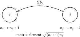
The transfer operator $b_i^\dagger b_j$ moves one boson from source mode $j$ to destination mode $i$. Its matrix element is $\sqrt{(n_i+1)n_j}$: the source factor requires a boson to remove, while the destination factor produces Bose enhancement. The mode occupations change, but the total $N=n_i+n_j+\cdots$ does not.

Bose enhancement

The factor $\sqrt{n_i+1}$ means that a transition into an already occupied bosonic mode has a larger amplitude than a transition into an empty mode, all else equal. The corresponding squared matrix element contains $n_i+1$.

This algebraic enhancement is not an attractive force. A transition rate also depends on the perturbation, energy conservation, density of final states, and environmental or driving assumptions. The commutation relation supplies the occupation factor, not an entire dynamical prediction.

The Mode Basis Is Part of the Model

A mode can be a localized lattice orbital, a momentum state, a trap eigenfunction, an internal atomic state, a phonon normal mode, a cavity resonance, or another orthonormal one-particle state. Its operator is

$$b_i^\dagger = \int dq\, \varphi_i(q) \psi^\dagger(q),$$

where $\varphi_i(q)$ is the mode wavefunction and $\psi^\dagger(q)$ is a field operator.

Under a unitary change of one-particle basis,

$$a_\alpha = \sum_i U_{\alpha i}b_i,$$

the new operators obey

$$[a_\alpha,a_\beta^\dagger] = \delta_{\alpha\beta}I.$$

The physical Hamiltonian is unchanged when both operators and coefficients are transformed consistently. Truncation can spoil this equivalence: projecting onto a finite set of localized orbitals and projecting onto a finite set of momentum modes generally define different approximations.

General One-Body Terms

A number-conserving one-body Hamiltonian has the form

$$H_1 = \sum_{i,j} h_{ij} b_i^\dagger b_j.$$

Hermiticity requires

$$h_{ij} = h_{ji}^*.$$

Diagonal terms measure occupations,

$$H_{\mathrm{diag}} = \sum_i \epsilon_i n_i,$$

whereas off-diagonal terms transfer bosons between modes. This is the mode-basis form of lifting a one-particle operator to Fock space; the general derivation lives in One-Body Operators.

Matrix element audit

For two configurations $\boldsymbol m$ and $\boldsymbol n$,

$$\begin{aligned} \langle\boldsymbol m\vert H_1 \vert\boldsymbol n\rangle &= \sum_{i,j} h_{ij} \sqrt{(n_i+1)n_j} \\ &\quad\times \delta_{\boldsymbol m, \boldsymbol n+\boldsymbol e_i-\boldsymbol e_j} \end{aligned}$$

for $i\ne j$, with diagonal $i=j$ terms contributing $h_{ii}n_i$. This formula is a useful implementation check because it separates the physical coefficient $h_{ij}$ from the universal bosonic square-root factor.

Hopping Hamiltonians

On a graph or lattice, a common bond convention is

$$\begin{aligned} H_t = -\sum_{\langle i,j\rangle} \bigl( J_{ij}b_i^\dagger b_j + J_{ij}^*b_j^\dagger b_i \bigr). \end{aligned}$$

Each unordered bond is counted once. The second term is the Hermitian conjugate of the first. For real uniform hopping,

$$H_t = -J \sum_{\langle i,j\rangle} \left( b_i^\dagger b_j + b_j^\dagger b_i \right).$$

The leading minus sign is conventional. Its physical consequences depend on lattice geometry, boundary conditions, and hopping phases. On some bipartite lattices it can be changed by a local phase transformation; in frustrated loops, gauge-invariant fluxes remain.

Hopping action

On one bond,

$$\begin{aligned} H_{t,ij} \lvert\ldots,n_i,n_j,\ldots\rangle ={}& -J_{ij} \sqrt{(n_i+1)n_j} \\ &\times \lvert\ldots,n_i+1,n_j-1,\ldots\rangle \\ &- J_{ij}^* \sqrt{n_i(n_j+1)} \\ &\times \lvert\ldots,n_i-1,n_j+1,\ldots\rangle. \end{aligned}$$

This one line gives the off-diagonal entries used by exact diagonalization, configuration-interaction methods, and occupation-space graph constructions.

Onsite Energies and Chemical Potential

An onsite energy or external potential contributes

$$H_\epsilon = \sum_i \epsilon_i n_i.$$

In a grand-canonical description, one works with

$$K = H-\mu N,$$

so the diagonal coefficient becomes $\epsilon_i-\mu$ for uniform particle chemical potential. The term $-\mu N$ does not break number conservation:

$$[K,N]=0$$

whenever $[H,N]=0$.

In a fixed-$N$ calculation, a uniform $-\mu N$ is a constant shift and can be omitted. Site-dependent chemical potentials or trap offsets are not constant within a fixed total-number sector.

Onsite Pair Interactions

The normally ordered onsite quartic operator satisfies

$$(b_i^\dagger)^2b_i^2 = n_i(n_i-1).$$

Indeed,

$$\begin{aligned} (b_i^\dagger)^2b_i^2 \lvert n_i\rangle &= n_i(n_i-1) \lvert n_i\rangle. \end{aligned}$$

The standard onsite interaction is therefore

$$H_U = \frac{U}{2} \sum_i n_i(n_i-1).$$

On a site with $n$ bosons, the energy is

$$E_U(n) = U\binom n2 = \frac{U}{2}n(n-1).$$

The factor counts unordered onsite pairs. It also makes the one-particle interaction energy vanish.

Why not simply use squared occupation?

Because

$$n_i^2 = n_i(n_i-1)+n_i,$$

replacing the pair term by $Un_i^2/2$ adds a one-body contribution $Un_i/2$. At fixed total $N$, summing this difference over all sites gives the constant $UN/2$. In a grand-canonical problem, it shifts the effective chemical potential and is not harmless unless conventions are adjusted.

General Two-Body Interactions

In an orthonormal mode basis, a number-conserving two-body interaction is

$$H_2 = \frac12 \sum_{i,j,k,l} V_{ij;kl} b_i^\dagger b_j^\dagger b_l b_k.$$

For unsymmetrized product-basis matrix elements of an exchange-symmetric interaction,

$$V_{ij;kl} = V_{ji;lk},$$

and Hermiticity requires

$$V_{ij;kl} = V_{kl;ij}^*.$$

Because bosonic creation operators commute with each other, and so do bosonic annihilation operators, only the coefficient part symmetric within each creation pair and annihilation pair contributes to the operator. Some references therefore define explicitly symmetrized matrix elements, for which additional index equalities hold.

Coefficient definitions differ across fields. A prefactor can move when matrix elements are pre-symmetrized or sums are restricted. The foundational lift lives in Two-Body Operators; the many-body application guide develops statistics-adapted coefficients, two-body density matrices, basis changes, and numerical checks.

Common Quartic Terms

Density-density interaction

For different modes,

$$H_V = \frac12 \sum_{i\ne j} V_{ij}n_i n_j,$$

with $V_{ij}=V_{ji}$. If unordered neighbors are summed once, write instead

$$H_V = \sum_{\langle i,j\rangle} V_{ij}n_i n_j.$$

Pair hopping

A pair can transfer between modes through

$$H_P = \sum_{i<j} \left[ P_{ij}(b_i^\dagger)^2b_j^2 + P_{ij}^*(b_j^\dagger)^2b_i^2 \right].$$

Its forward matrix element contains

$$\sqrt{ (n_i+1)(n_i+2) n_j(n_j-1) }.$$

The source mode must contain at least two bosons.

Density-assisted hopping

Effective models can contain terms such as

$$b_i^\dagger n_j b_j.$$

Operator order matters when a number operator shares a mode with a ladder operator. For example,

$$n_j b_j \ne b_j n_j.$$

Use commutators or act on number states rather than treating all symbols as commuting scalars.

Number Conservation and U(1) Symmetry

The total number operator obeys

$$[N,b_i] = -b_i, \qquad [N,b_i^\dagger] = b_i^\dagger.$$

For a normally ordered monomial with $p$ creation and $q$ annihilation operators,

$$[N,M_{p,q}] = (p-q)M_{p,q}.$$

Therefore equal numbers of creation and annihilation operators imply

$$[N,H]=0.$$

Such a Hamiltonian is invariant under the global phase transformation

$$b_i \longmapsto e^{i\theta}b_i, \qquad b_i^\dagger \longmapsto e^{-i\theta}b_i^\dagger.$$

This is the global $U(1)$ symmetry associated with particle-number conservation.

Conservation under a Hamiltonian is not, by itself, a universal superselection rule. It states that the dynamics does not mix number sectors.

Number-Changing Terms

A coherent source has the form

$$H_{\mathrm{src}} = \sum_i \left( f_i b_i^\dagger + f_i^* b_i \right).$$

It changes particle number by one and explicitly breaks the global $U(1)$ symmetry of the isolated bosonic subsystem. Physically, it can describe exchange with a phase-referenced drive or a symmetry-breaking probe.

A quadratic pairing term is

$$H_{\mathrm{pair}} = \frac12 \sum_{i,j} \left( \Delta_{ij}b_i^\dagger b_j^\dagger + \Delta_{ij}^*b_jb_i \right).$$

It changes $N$ by two, so number parity can remain conserved even though $N$ does not. Such terms arise in effective descriptions and Bogoliubov theories; stability requires checking the full quadratic Hamiltonian, not the pairing block alone.

Bond Current

For the hopping bond

$$H_{t,ij} = -J_{ij}b_i^\dagger b_j -J_{ij}^*b_j^\dagger b_i,$$

define current from $i$ to $j$ by the contribution to

$$\frac{dn_i}{dt} = -I_{i\to j}.$$

The Heisenberg equation gives

$$I_{i\to j} = -\frac{i}{\hbar} \left( J_{ij}b_i^\dagger b_j - J_{ij}^*b_j^\dagger b_i \right).$$

Thus

$$\langle I_{i\to j}\rangle = \frac{2}{\hbar} \operatorname{Im} \left[ J_{ij} \langle b_i^\dagger b_j\rangle \right].$$

The sign depends on the chosen bond orientation. A later density-and-current page owns the full continuity-equation treatment; here the formula shows that hopping coherence, not occupation alone, carries particle current.

Complex Hopping and Gauge Choice

Write

$$J_{ij} = |J_{ij}|e^{iA_{ij}}.$$

Under a local mode rephasing

$$b_i \longmapsto e^{i\chi_i}b_i,$$

the coefficient representation changes as

$$J_{ij} \longmapsto e^{i(\chi_i-\chi_j)}J_{ij}.$$

Individual bond phases are basis dependent. The accumulated phase around a closed loop is gauge invariant modulo $2\pi$ and can encode synthetic magnetic flux or frustration.

Changing the sign of one hopping coefficient is therefore sometimes a gauge convention and sometimes a physical flux change. The graph topology decides which.

Bose–Hubbard Assembly Example

The standard single-component Bose–Hubbard grand Hamiltonian is

$$\begin{aligned} K_{\mathrm{BH}} ={}& -J \sum_{\langle i,j\rangle} \left( b_i^\dagger b_j + b_j^\dagger b_i \right) \\ &+ \frac{U}{2} \sum_i n_i(n_i-1) \\ &+ \sum_i (\epsilon_i-\mu)n_i. \end{aligned}$$

Each term has a distinct operator role:

Term	Operator action	Physical role
$-Jb_i^\dagger b_j+\mathrm{h.c.}$	moves one boson across a bond	delocalization and phase coherence
$Un_i(n_i-1)/2$	counts onsite pairs	repulsion for $U>0$, attraction for $U<0$
$\epsilon_i n_i$	weights site occupation	trap, disorder, or sublattice offset
$-\mu n_i$	weights total number sectors	grand-canonical control of filling

The full conventions, limits, and phase-boundary preview live in the Bose–Hubbard Model; the model card is the compact lookup entry. Quantum Phase Transitions owns the generic superfluid–Mott critical interpretation. This page owns how the operator terms act and how to audit them.

Limiting checks

• At $J=0$, every occupation vector is an eigenstate.
• At $U=0$, the Hamiltonian is quadratic and can be diagonalized by a one-particle basis transformation.
• At fixed total $N$, uniform $-\mu N$ is a constant.
• For $N=1$, the onsite interaction vanishes identically.
• For real $J$, the Hamiltonian matrix is real symmetric in the occupation basis.

Two-site action without rebuilding the full matrix

For two bosons and real hopping,

$$\begin{aligned} H_t\lvert1,1\rangle &= -\sqrt2J \left( \lvert2,0\rangle + \lvert0,2\rangle \right). \end{aligned}$$

The $\sqrt2$ factors are Bose enhancement at the destination modes. The full fixed-$N=2$ matrix and its sparse-basis construction live in Occupation-Number Representation.

Multi-Component Bosons

For internal component $\alpha$,

$$[b_{i\alpha},b_{j\beta}^\dagger] = \delta_{ij}\delta_{\alpha\beta}I.$$

The component occupation is

$$n_{i\alpha} = b_{i\alpha}^\dagger b_{i\alpha}.$$

A general onsite density interaction can be written

$$H_{\mathrm{int}} = \frac12 \sum_{i,\alpha,\beta} U_{\alpha\beta} b_{i\alpha}^\dagger b_{i\beta}^\dagger b_{i\beta} b_{i\alpha}.$$

For $\alpha=\beta$, this produces $n_{i\alpha}(n_{i\alpha}-1)$. For distinct components and symmetric $U_{\alpha\beta}$, it produces $U_{\alpha\beta}n_{i\alpha}n_{i\beta}$ after the prefactor and duplicate component orderings are combined.

Conversion terms can conserve total number while changing component populations. For example,

$$g (b_{i\uparrow}^\dagger)^2 b_{i\downarrow}^2 + g^* (b_{i\downarrow}^\dagger)^2 b_{i\uparrow}^2$$

converts pairs between internal states. The conserved charges must be determined from the actual term, not inferred from the presence of component labels.

Momentum-Space Preview

For $L$ periodic lattice sites at positions $\mathbf R_j$, define

$$b_{\mathbf k} = \frac1{\sqrt L} \sum_j e^{-i\mathbf k\cdot\mathbf R_j} b_j.$$

The transformed operators obey canonical bosonic commutators. Translation-invariant quadratic hopping becomes diagonal,

$$H_t = \sum_{\mathbf k} \varepsilon(\mathbf k) b_{\mathbf k}^\dagger b_{\mathbf k},$$

while local interactions become quartic momentum sums with total crystal momentum conserved modulo a reciprocal lattice vector.

This illustrates a recurring tradeoff: a basis that diagonalizes hopping makes local interactions nonlocal in mode labels. Momentum-Space Representation owns the systematic transform and normalization conventions.

Hard-Core Bosons Are Projected Bosons

A hard-core boson mode allows only

$$n_i\in\{0,1\}.$$

Let $\widetilde b_i$ denote the operator projected into that two-dimensional local space. Then

$$\widetilde b_i^2 = 0,$$

and, on the same site,

$$[\widetilde b_i,\widetilde b_i^\dagger] = I-2n_i.$$

This is not the canonical bosonic commutator. Operators on distinct sites still commute in the standard hard-core-boson construction.

The local mapping

$$\widetilde b_i \longleftrightarrow S_i^-, \qquad \widetilde b_i^\dagger \longleftrightarrow S_i^+, \qquad n_i \longleftrightarrow S_i^z+\frac12$$

relates hard-core lattice bosons to spin-$1/2$ models. Calling them “bosons” refers to their intersite exchange structure and lattice-particle interpretation, not to a canonical onsite oscillator algebra.

Numerical Occupation Cutoffs

Canonical bosonic Fock space has unbounded local occupation. A calculation may impose

$$0\le n_i\le n_{\max}.$$

If creation is projected to vanish at the top state, the finite local matrices satisfy

$$[b_i,b_i^\dagger]_{\mathrm{trunc}} = I -(n_{\max}+1) \lvert n_{\max}\rangle \langle n_{\max}\rvert.$$

The canonical commutator fails only at the truncation boundary, but that failure matters if the state has appreciable weight there.

A controlled calculation should report at least one cutoff diagnostic, such as

$$P(n_i=n_{\max})$$

or convergence of observables under $n_{\max}\to n_{\max}+1$. A low mean occupation does not alone prove that the cutoff tail is negligible.

Stability Checks

Because bosonic occupation is unbounded, coefficient signs can determine whether a model has a lower-bounded energy.

For example, a single grand-canonical mode with only

$$-\frac{|U|}{2}n(n-1) -\mu n$$

is unbounded below as $n\to\infty$. A finite numerical cutoff can hide this instability by turning the top basis state into an artificial ground state.

At fixed finite total $N$, an attractive lattice Hamiltonian can be bounded within that sector, but its energy may fail to be extensive or stable as $N$ grows. Effective three-body repulsion, loss, finite-range physics, or a restricted validity regime may be essential in a physical model.

For quadratic bosonic Hamiltonians with pairing, diagonalizing the coefficient matrix as if it were an ordinary Hermitian one-particle problem is insufficient. Bogoliubov Theory develops the paraunitary structure, metric normalization, and stability test.

Mean-Field Replacement Is an Approximation

Bosonic mean-field theory often writes

$$b_i = \phi_i + \delta b_i, \qquad \phi_i = \langle b_i\rangle.$$

Keeping only c-number fields or low-order fluctuations can be powerful, but it is not an operator identity. Replacing $b_i$ by a complex number discards commutators and quantum fluctuations.

In an exact finite system with a number-conserving Hamiltonian and a state of definite $N$,

$$\langle b_i\rangle = 0$$

because $b_i$ connects different number sectors. Condensation or phase coherence can instead be diagnosed through the one-body density matrix

$$\langle b_i^\dagger b_j\rangle.$$

A nonzero order parameter $\phi_i$ is obtained after introducing a phase reference, a symmetry-breaking source, or an appropriate thermodynamic-limit construction. Bose–Einstein Condensation owns the condensation criterion.

Operator Signatures of Common Observables

Bosonic models are often organized around a small set of expectation values:

Observable	Operator expression	Interpretation
mean occupation	$\langle n_i\rangle$	local population
number fluctuation	$\langle n_i^2\rangle-\langle n_i\rangle^2$	local compressibility or number squeezing context
first-order coherence	$\langle b_i^\dagger b_j\rangle$	phase coherence and one-body density matrix
onsite pair count	$\langle n_i(n_i-1)\rangle$	two-boson coincidence weight
anomalous amplitude	$\langle b_i b_j\rangle$	pairing relative to a number-breaking reference
bond current	$\langle I_{i\to j}\rangle$	directed transport under a stated convention

No single expectation value identifies a phase without limits, geometry, and symmetry assumptions. For example, finite-size coherence is not by itself proof of spontaneous symmetry breaking.

Building a Sparse Hamiltonian Reliably

1. Declare the mode basis. State whether indices label sites, momenta, orbitals, bands, spin components, or normal modes.
2. Choose the sector. Fix total $N$ or include all required number sectors.
3. Declare local cutoffs. Record $n_{\max}$ and convergence diagnostics.
4. Normal-order terms consistently. This makes number-state action and vacuum contributions explicit.
5. Add Hermitian conjugates. Do not rely on an informal “reverse process” unless it is written into the implementation.
6. Apply operators right to left. Update occupation factors after each operation.
7. Accumulate duplicate destinations. Distinct algebraic terms can connect the same pair of configurations.
8. Check conserved charges. Matrix blocks should agree with commutator analysis.
9. Test small systems analytically. One- and two-boson sectors expose most square-root and pair-counting errors.
10. Check limiting cases. Turn off hopping, interactions, sources, and pairing terms separately.

Common Mistakes

• Writing $b_i^\dagger$ without defining the mode $i$.
• Forgetting the factors $\sqrt{n_i}$ and $\sqrt{n_i+1}$.
• Treating Bose enhancement as an attractive interaction.
• Calling $b_i^\dagger b_j$ Hermitian without adding its conjugate when $i\ne j$.
• Counting an unordered hopping bond twice.
• Omitting the factor $1/2$ in an onsite pair interaction.
• Replacing $n_i(n_i-1)$ by $n_i^2$ without tracking the induced one-body shift.
• Assuming every quartic term conserves each component number.
• Treating hard-core bosons as canonical onsite oscillators.
• Assuming a finite occupation cutoff preserves $[b_i,b_i^\dagger]=I$ exactly.
• Trusting an attractive bosonic Hamiltonian without checking boundedness.
• Replacing operators by c-numbers without declaring a mean-field approximation.
• Inferring absence of condensation from $\langle b_i\rangle=0$ in a fixed-number finite system.
• Diagonalizing a bosonic pairing Hamiltonian with an ordinary unitary transformation only.

Summary

• Bosonic ladder operators act on declared modes and carry occupation-dependent square-root factors.
• Bilinears $b_i^\dagger b_j$ build one-body transfer and hopping terms.
• Quartic monomials build pair interactions, density couplings, pair hopping, and conversion processes.
• Hermiticity, pair-counting conventions, and operator order must be checked explicitly.
• Equal numbers of creation and annihilation operators imply total-number conservation and global $U(1)$ symmetry.
• Hopping coherence determines bond current under a stated orientation convention.
• The Bose–Hubbard model assembles hopping, onsite pairs, potentials, and chemical potential into one standard example.
• Hard-core projection and numerical occupation cutoffs modify the onsite commutator.
• Unbounded bosonic occupation makes stability and cutoff convergence essential checks.
• Mean-field c-number replacement is an approximation, not the bosonic algebra itself.

Exercises

Exercise 1: Transfer amplitudes

For two modes in the state $\lvert n_i=2,n_j=3\rangle$, compute

$$b_i^\dagger b_j \lvert2,3\rangle$$

and

$$b_j^\dagger b_i \lvert2,3\rangle.$$

Solution

For transfer from $j$ to $i$,

$$\sqrt{(n_i+1)n_j} = \sqrt{3\cdot3} = 3,$$

so

$$b_i^\dagger b_j \lvert2,3\rangle = 3\lvert3,2\rangle.$$

For the reverse transfer,

$$\sqrt{n_i(n_j+1)} = \sqrt{2\cdot4} = 2\sqrt2,$$

and therefore

$$b_j^\dagger b_i \lvert2,3\rangle = 2\sqrt2\lvert1,4\rangle.$$

Exercise 2: Onsite pair identity

Prove from $[b,b^\dagger]=I$ that

$$(b^\dagger)^2b^2 = n(n-1), \qquad n=b^\dagger b.$$

Solution

Start with

$$n^2 = b^\dagger b b^\dagger b.$$

Using

$$bb^\dagger = b^\dagger b+I,$$

gives

$$\begin{aligned} n^2 &= b^\dagger (b^\dagger b+I) b \\ &= (b^\dagger)^2b^2 + n. \end{aligned}$$

Rearranging yields

$$(b^\dagger)^2b^2 = n^2-n = n(n-1).$$

Exercise 3: Charge counting by commutators

Determine which terms conserve total number $N$:

$$b_i^\dagger b_j, \qquad (b_i^\dagger)^2b_j^2, \qquad b_i^\dagger b_j^\dagger, \qquad b_i^\dagger n_j b_k.$$

Solution

For a monomial, $[N,M]=(p-q)M$, where $p$ and $q$ count creation and annihilation operators. Number operators contain one of each and contribute zero net charge.

Thus

$$[N,b_i^\dagger b_j] = 0,$$

and

$$[N,(b_i^\dagger)^2b_j^2] = 0.$$

Pair creation has

$$[N,b_i^\dagger b_j^\dagger] = 2b_i^\dagger b_j^\dagger,$$

so it does not conserve $N$. Finally, $b_i^\dagger n_j b_k$ has one net creation and one net annihilation, hence

$$[N,b_i^\dagger n_j b_k] = 0.$$

Exercise 4: Hermiticity and bond current

Let

$$H_{ij} = -Jb_i^\dagger b_j -J^*b_j^\dagger b_i.$$

Show that $H_{ij}$ is Hermitian and derive the contribution to $dn_i/dt$.

Solution

Taking the adjoint exchanges the two terms:

$$H_{ij}^\dagger = -J^*b_j^\dagger b_i -Jb_i^\dagger b_j = H_{ij}.$$

The needed commutators are

$$[b_i^\dagger b_j,n_i] = -b_i^\dagger b_j,$$

and

$$[b_j^\dagger b_i,n_i] = b_j^\dagger b_i.$$

Therefore

$$\begin{aligned} \frac{dn_i}{dt} &= \frac{i}{\hbar}[H_{ij},n_i] \\ &= \frac{i}{\hbar} \left( Jb_i^\dagger b_j -J^*b_j^\dagger b_i \right). \end{aligned}$$

Defining current from $i$ to $j$ by $dn_i/dt=-I_{i\to j}$ gives the expression used in the text.

Exercise 5: Two-site Bose–Hubbard action

For

$$H = -J (b_1^\dagger b_2+b_2^\dagger b_1) + \frac U2 \sum_{i=1}^{2} n_i(n_i-1),$$

compute $H\lvert2,0\rangle$ and $H\lvert1,1\rangle$.

Solution

For $\lvert2,0\rangle$, only transfer from site $1$ to site $2$ is possible:

$$b_2^\dagger b_1 \lvert2,0\rangle = \sqrt2\lvert1,1\rangle.$$

There is one onsite pair on site $1$, so

$$H\lvert2,0\rangle = U\lvert2,0\rangle - \sqrt2J\lvert1,1\rangle.$$

For $\lvert1,1\rangle$, there are no onsite pairs, and either boson can hop into the occupied destination mode:

$$H\lvert1,1\rangle = -\sqrt2J \left( \lvert2,0\rangle + \lvert0,2\rangle \right).$$

Exercise 6: Hard-core mapping

Using

$$\widetilde b=S^- , \qquad \widetilde b^\dagger=S^+, \qquad n=S^z+\frac12,$$

show that the hard-core commutator equals $I-2n$.

Solution

Spin operators obey

$$[S^+,S^-] = 2S^z,$$

so

$$[S^-,S^+] = -2S^z.$$

Using $n=S^z+1/2$,

$$I-2n = I-2S^z-I = -2S^z.$$

Therefore

$$[\widetilde b,\widetilde b^\dagger] = [S^-,S^+] = I-2n.$$

Exercise 7: Truncated commutator

Let a projected oscillator retain $\lvert0\rangle,\ldots,\lvert n_{\max}\rangle$ and set $b^\dagger\lvert n_{\max}\rangle=0$. Verify

$$[b,b^\dagger]_{\mathrm{trunc}} = I -(n_{\max}+1) \lvert n_{\max}\rangle \langle n_{\max}\rvert.$$

Solution

For $0\le n<n_{\max}$, both ladder operations remain inside the retained space, so

$$[b,b^\dagger]\lvert n\rangle = \lvert n\rangle.$$

At the top state,

$$bb^\dagger\lvert n_{\max}\rangle = 0,$$

while

$$b^\dagger b\lvert n_{\max}\rangle = n_{\max}\lvert n_{\max}\rangle.$$

Hence the commutator eigenvalue there is $-n_{\max}$. The proposed operator has top-state eigenvalue

$$1-(n_{\max}+1) = -n_{\max},$$

and eigenvalue $1$ on every lower retained state, proving the identity.

Exercise 8: Detecting an artificial cutoff ground state

Consider one mode with

$$K = -\frac{|U|}{2}n(n-1) -\mu n.$$

Explain why a calculation with cutoff $n\le n_{\max}$ tends to place the ground state at the cutoff for sufficiently large $n_{\max}$. What does this imply about the untruncated model?

Solution

The number-state energy is

$$E_n = -\frac{|U|}{2}n(n-1) -\mu n.$$

The negative quadratic term dominates at large $n$, so $E_n\to-\infty$. In a finite truncated basis, the lowest available energy therefore eventually occurs at or near $n=n_{\max}$.

Increasing the cutoff moves the apparent ground state and lowers its energy without convergence. This is not evidence for a highly occupied stable phase; it diagnoses that the untruncated Hamiltonian is unbounded below. Stabilizing physics or a restricted fixed-number sector must be supplied before the model is physically complete.

References

• A. L. Fetter and J. D. Walecka, Quantum Theory of Many-Particle Systems, Dover (2003).
• J. W. Negele and H. Orland, Quantum Many-Particle Systems, Westview Press (1998).
• P. Coleman, Introduction to Many-Body Physics, Cambridge University Press (2015).
• A. Altland and B. Simons, Condensed Matter Field Theory, 2nd ed., Cambridge University Press (2010).
• S. Sachdev, Quantum Phase Transitions, 2nd ed., Cambridge University Press (2011).
• A. Auerbach, Interacting Electrons and Quantum Magnetism, Springer (1994).
• M. P. A. Fisher, P. B. Weichman, G. Grinstein, and D. S. Fisher, “Boson localization and the superfluid-insulator transition,” Physical Review B 40, 546–570 (1989), doi:10.1103/PhysRevB.40.546.
• D. Jaksch, C. Bruder, J. I. Cirac, C. W. Gardiner, and P. Zoller, “Cold bosonic atoms in optical lattices,” Physical Review Letters 81, 3108–3111 (1998), doi:10.1103/PhysRevLett.81.3108.
• I. Bloch, J. Dalibard, and W. Zwerger, “Many-body physics with ultracold gases,” Reviews of Modern Physics 80, 885–964 (2008), doi:10.1103/RevModPhys.80.885.