Field-Operator Applications

Nonrelativistic field operators turn mode-based many-body mechanics into a spatial language. The annihilation field $\psi(x)$ removes one particle from the one-particle state localized at $x$, while $\psi^\dagger(x)$ creates one. Here $x$ may combine position and an internal label such as spin.

For a one-particle basis $\{\varphi_i(x)\}$,

$$\begin{aligned} \psi(x) &= \sum_i \varphi_i(x)a_i, \\ \psi^\dagger(x) &= \sum_i \varphi_i^*(x)a_i^\dagger. \end{aligned}$$

This is not a new physical theory. It is the position-space representation of the same Fock-space operators used in the occupation-number description.

The Many-Body Hilbert Spaces Overview distinguishes the physical state space from a field-operator representation of it. The canonical definitions, distributional meaning, and equal-time algebra live in Field Operators and Mode Expansions. This page owns their deployment in continuum many-body models, contact and nonlocal interactions, fixed-particle reconstruction, regularization cautions, and the boundary with QFT. The complete spatial and Fourier dictionaries live in Real-Space Representation and Momentum-Space Representation.

Conventions

Unless stated otherwise:

• space has dimension $d$;
• fields are in the Schrödinger picture and evaluated at a common time;
• $x=(\mathbf r,\sigma)$ includes position and any discrete internal label;
• integration over $x$ means

$$\int dx \equiv \sum_\sigma \int d^dr;$$

• the one-particle modes are orthonormal and complete in the stated model space;
• boundary conditions are declared when integrations by parts or Fourier modes are used.

For a spinless field, the label $\sigma$ and its sum are absent.

Fields Are Operator-Valued Distributions

The symbol $\psi(\mathbf r)$ is not an ordinary bounded operator at an exact point. It is an operator-valued distribution. The controlled object is a smeared field

$$\psi[f] = \int d^dr\, f^*(\mathbf r) \psi(\mathbf r),$$

with adjoint

$$\psi^\dagger[f] = \int d^dr\, f(\mathbf r) \psi^\dagger(\mathbf r).$$

For normalized $f$,

$$\psi^\dagger[f]\lvert0\rangle$$

is the one-particle state with wavefunction $f$. Unsmeared formulas are compact distributional notation whose meaning is fixed by integration against wavepackets or other test functions.

A Unified Equal-Time Bracket

Define

$$[A,B]_\eta \equiv AB-\eta BA,$$

with

$$\eta = \begin{cases} +1, & \text{bosons}, \\ -1, & \text{fermions}. \end{cases}$$

The equal-time field algebra is

$$[\psi(x),\psi^\dagger(x')]_\eta = \delta(x-x'),$$

and

$$[\psi(x),\psi(x')]_\eta = 0.$$

The combined delta means

$$\delta(x-x') = \delta_{\sigma\sigma'} \delta^{(d)} (\mathbf r-\mathbf r').$$

For smeared fields,

$$[\psi[f],\psi^\dagger[g]]_\eta = \langle f\vert g\rangle.$$

This last equation is an ordinary operator identity and makes the distributional interpretation explicit.

Mode Expansion and Inverse Projection

Let

$$\int dx\, \varphi_i^*(x) \varphi_j(x) = \delta_{ij}.$$

Completeness means

$$\sum_i \varphi_i(x) \varphi_i^*(x') = \delta(x-x').$$

The field expansion and its inverse are

$$\begin{aligned} \psi(x) &= \sum_i \varphi_i(x)a_i, \\ a_i &= \int dx\, \varphi_i^*(x) \psi(x). \end{aligned}$$

Likewise,

$$\begin{aligned} \psi^\dagger(x) &= \sum_i \varphi_i^*(x)a_i^\dagger, \\ a_i^\dagger &= \int dx\, \varphi_i(x) \psi^\dagger(x). \end{aligned}$$

The complex conjugation follows from taking the adjoint. Losing it is one of the most common mode-expansion errors.

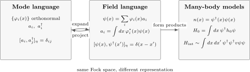
The mode and field descriptions are equivalent when the one-particle basis is complete. Expanding mode operators produces a spatial field; projecting the field onto a mode recovers the corresponding annihilation or creation operator. Local densities and continuum Hamiltonians are field-operator products built from the same Fock-space algebra.

Recovering the Delta Algebra

Substitution of the mode expansion gives

$$\begin{aligned} [\psi(x),\psi^\dagger(x')]_\eta &= \sum_{i,j} \varphi_i(x) \varphi_j^*(x') [a_i,a_j^\dagger]_\eta \\ &= \sum_i \varphi_i(x) \varphi_i^*(x') \\ &= \delta(x-x'). \end{aligned}$$

The first equality uses the mode algebra; the last uses completeness. In a truncated mode space, the final sum is a projection kernel rather than an exact Dirac delta.

What Local Annihilation Means

For any Fock-space state $\lvert\Psi\rangle$,

$$\psi(x)\lvert\Psi\rangle$$

is a state with one fewer particle. Its squared norm is

$$\left\lVert \psi(x)\lvert\Psi\rangle \right\rVert^2 = \langle\Psi\vert \psi^\dagger(x)\psi(x) \vert\Psi\rangle.$$

The right-hand side is the expected number density at $x$. This gives operational meaning to the phrase “annihilate a particle at $x$” without treating $\psi(x)$ as a one-particle wavefunction.

Reconstructing a Fixed-N Wavefunction

Let $\Psi_N(x_1,\ldots,x_N)$ be normalized and symmetric for bosons or antisymmetric for fermions. The corresponding fixed-$N$ Fock state is

$$\begin{aligned} \lvert\Psi_N\rangle ={}& \frac{1}{\sqrt{N!}} \int dx_1\cdots dx_N \\ &\times \Psi_N(x_1,\ldots,x_N) \\ &\times \psi^\dagger(x_1) \cdots \psi^\dagger(x_N) \lvert0\rangle. \end{aligned}$$

The inverse relation is

$$\begin{aligned} \Psi_N(x_1,\ldots,x_N) ={}& \frac{1}{\sqrt{N!}} \\ &\times \langle0\vert \psi(x_N) \cdots \psi(x_1) \\ &\times \lvert\Psi_N\rangle. \end{aligned}$$

The ordering in the inverse formula is important for fermions. Exchange symmetry or antisymmetry follows from the field algebra.

Acting once with the annihilation field produces an $(N-1)$-particle state whose coordinate wavefunction is proportional to

$$\sqrt N\, \Psi_N(x,x_2,\ldots,x_N).$$

Thus the field formalism and first quantization agree sector by sector.

One-Body Continuum Hamiltonians

Let the one-particle Hamiltonian be

$$h_0 = -\frac{\hbar^2}{2m}\nabla^2 + V_{\mathrm{ext}}(\mathbf r).$$

Its many-body lift is

$$H_0 = \int d^dr\, \psi^\dagger(\mathbf r) h_0 \psi(\mathbf r).$$

The differential operator acts on the field to its right. Under boundary conditions that remove surface terms, the kinetic energy can also be written

$$T = \frac{\hbar^2}{2m} \int d^dr\, \nabla\psi^\dagger \boldsymbol\cdot \nabla\psi.$$

For fields with internal components,

$$H_0 = \sum_{\sigma,\sigma'} \int d^dr\, \psi_\sigma^\dagger(\mathbf r) [h_0]_{\sigma\sigma'} \psi_{\sigma'}(\mathbf r).$$

The matrix $[h_0]_{\sigma\sigma'}$ may contain spin coupling, Zeeman terms, spin-orbit coupling, or other one-body internal structure.

Returning to a Discrete One-Body Matrix

Insert the mode expansion into the continuum one-body Hamiltonian. The result is

$$H_0 = \sum_{i,j} h_{ij} a_i^\dagger a_j,$$

where

$$h_{ij} = \int dx\, \varphi_i^*(x) h_0 \varphi_j(x).$$

If the modes diagonalize $h_0$, then

$$h_{ij} = \epsilon_i\delta_{ij},$$

and

$$H_0 = \sum_i \epsilon_i a_i^\dagger a_i.$$

The field and mode forms therefore encode the same one-body operator. One is spatially transparent; the other may be computationally or spectrally convenient.

Nonlocal Two-Body Interactions

For a symmetric pair potential $v(x,x')$, the number-conserving interaction is

$$\begin{aligned} H_{\mathrm{int}} ={}& \frac12 \int dx\,dx'\, \psi^\dagger(x) \psi^\dagger(x') \\ &\times v(x,x') \psi(x') \psi(x). \end{aligned}$$

The factor $1/2$ prevents double counting unordered pairs. The annihilation order is part of the convention and must be kept fixed for fermions.

Expansion in modes gives

$$H_{\mathrm{int}} = \frac12 \sum_{i,j,k,l} V_{ij;kl} a_i^\dagger a_j^\dagger a_l a_k,$$

with

$$\begin{aligned} V_{ij;kl} ={}& \int dx\,dx'\, \varphi_i^*(x) \varphi_j^*(x') \\ &\times v(x,x') \varphi_k(x) \varphi_l(x'). \end{aligned}$$

This is the continuum origin of the standard two-body matrix elements used in occupation-space calculations.

Bosonic Contact Interaction

For a spinless bosonic field, a zero-range effective interaction is written

$$H_{\mathrm{contact}}^{(B)} = \frac{g_B}{2} \int d^dr\, \psi^\dagger \psi^\dagger \psi \psi.$$

Every field in the integrand is evaluated at the same position. Equivalently,

$$H_{\mathrm{contact}}^{(B)} = \frac{g_B}{2} \int d^dr\, {:}n^2(\mathbf r){:},$$

where

$$n(\mathbf r) = \psi^\dagger(\mathbf r) \psi(\mathbf r).$$

Normal ordering removes the self-contraction implicit in $n^2$, but it does not by itself solve every ultraviolet problem of a continuum contact theory.

The Weakly Interacting Bose Gas Preview uses this operator model to identify the dilute parameter, mean-field equation of state, healing scale, and Bogoliubov excitation spectrum.

Two-Component Fermionic Contact Interaction

For two fermionic components, a standard intercomponent contact term is

$$\begin{aligned} H_{\mathrm{contact}}^{(F)} = g_F \int d^dr\, &\psi_\uparrow^\dagger \psi_\downarrow^\dagger \\ &\times \psi_\downarrow \psi_\uparrow. \end{aligned}$$

No factor $1/2$ appears because the displayed term counts one ordered pair of distinct components. An equivalent spin-summed expression may use $1/2$ and sum over both component orders.

A same-component zero-range $s$-wave term vanishes formally because

$$\psi_\sigma(\mathbf r) \psi_\sigma(\mathbf r) = 0,$$

but this should be interpreted with the same distributional and regularization care as every coincident-point identity. Identical fermions can still interact through finite-range forces and higher partial waves.

Representative Continuum Models

Trapped bosons

A standard dilute-boson Hamiltonian is

$$\begin{aligned} H_B ={}& \int d^dr\, \psi^\dagger \left( -\frac{\hbar^2\nabla^2}{2m} + V_{\mathrm{ext}} \right) \psi \\ &+ \frac{g_B}{2} \int d^dr\, \psi^\dagger \psi^\dagger \psi \psi. \end{aligned}$$

The ideal gas is recovered at $g_B=0$. Replacing the operator field by a classical order-parameter field is a mean-field approximation, not an identity.

Two-component fermions

For two equal-mass components,

$$\begin{aligned} H_F ={}& \sum_{\sigma=\uparrow,\downarrow} \int d^dr\, \psi_\sigma^\dagger h_0 \psi_\sigma \\ &+ g_F \int d^dr\, \psi_\uparrow^\dagger \psi_\downarrow^\dagger \psi_\downarrow \psi_\uparrow. \end{aligned}$$

This is an effective low-energy model. The relation between $g_F$, the scattering length, and a regulator must be specified before quantitative continuum calculations are trustworthy.

Finite-Volume Momentum Expansion

In a periodic box of volume $V=L^d$,

$$\psi(\mathbf r) = \frac{1}{\sqrt V} \sum_{\mathbf k} e^{i\mathbf k\cdot\mathbf r} a_{\mathbf k},$$

with

$$\mathbf k = \frac{2\pi}{L} \mathbf n, \qquad \mathbf n \in \mathbb Z^d.$$

The inverse is

$$a_{\mathbf k} = \frac{1}{\sqrt V} \int_V d^dr\, e^{-i\mathbf k\cdot\mathbf r} \psi(\mathbf r).$$

The kinetic Hamiltonian becomes diagonal:

$$T = \sum_{\mathbf k} \frac{\hbar^2k^2}{2m} a_{\mathbf k}^\dagger a_{\mathbf k}.$$

The box normalization and the continuum normalization must not be mixed. The Fourier-transform conventions page owns the site-wide choices, while Momentum-Space Representation develops the complete many-body box-to-continuum dictionary.

Contact Interaction in Momentum Space

For periodic spinless bosons,

$$\begin{aligned} H_{\mathrm{contact}}^{(B)} ={}& \frac{g_B}{2V} \sum_{\mathbf k_1,\mathbf k_2,\mathbf q} a_{\mathbf k_1+\mathbf q}^\dagger a_{\mathbf k_2-\mathbf q}^\dagger \\ &\times a_{\mathbf k_2} a_{\mathbf k_1}. \end{aligned}$$

The momentum transfer is $\mathbf q$. Each term conserves total momentum because

$$(\mathbf k_1+\mathbf q) + (\mathbf k_2-\mathbf q) = \mathbf k_1+\mathbf k_2.$$

For a translationally invariant nonlocal potential, $g_B$ is replaced by its Fourier transform $\widetilde v(\mathbf q)$.

Projection onto Lattice Orbitals

Let $w_i(\mathbf r)$ be localized orthonormal orbitals. A single-band projection writes

$$\psi_\sigma(\mathbf r) \approx \sum_i w_i(\mathbf r) c_{i\sigma}.$$

The approximation sign records the discarded bands or orbitals. The one-body matrix elements are

$$t_{ij} = \int d^dr\, w_i^*(\mathbf r) h_0 w_j(\mathbf r).$$

For a strongly localized contact interaction, the dominant onsite coefficient is

$$U = g \int d^dr\, \lvert w_i(\mathbf r)\rvert^4.$$

This projection produces lattice hopping and onsite-interaction terms after additional approximations are stated. The continuum field and lattice operators are not different particle species; they are descriptions at different resolutions.

Density and Correlation Previews

The local number-density operator is

$$n(x) = \psi^\dagger(x) \psi(x),$$

and the total number is

$$N = \int dx\, n(x).$$

The one-body density matrix is

$$G^{(1)}(x,x') = \left\langle \psi^\dagger(x) \psi(x') \right\rangle.$$

At equal points,

$$G^{(1)}(x,x) = \langle n(x)\rangle.$$

Four-field products probe pair correlations. Their ordering, connected parts, and time dependence belong to the dedicated correlation-function pages; a mean density alone does not determine them.

Heisenberg Equation for a Bosonic Contact Model

For the trapped-boson Hamiltonian, the exact operator equation is

$$\begin{aligned} i\hbar \frac{\partial\psi}{\partial t} ={}& \left( -\frac{\hbar^2\nabla^2}{2m} + V_{\mathrm{ext}} \right) \psi \\ &+ g_B \psi^\dagger \psi \psi. \end{aligned}$$

Every field is evaluated at $(\mathbf r,t)$. This is an operator equation. Replacing $\psi$ by a complex function and factorizing correlations produces a Gross–Pitaevskii-type mean-field equation under additional assumptions.

Global U(1) Symmetry and Number Conservation

The number operator satisfies

$$\begin{aligned} [N,\psi(x)] &= -\psi(x), \\ [N,\psi^\dagger(x)] &= \psi^\dagger(x). \end{aligned}$$

Therefore

$$e^{i\theta N} \psi(x) e^{-i\theta N} = e^{-i\theta} \psi(x).$$

A number-conserving Hamiltonian is invariant under this global phase rotation and obeys

$$[H,N] = 0.$$

Pairing terms such as $\psi^\dagger\psi^\dagger+\psi\psi$ break particle-number U(1) symmetry in an effective description, though fermion parity may remain conserved.

Engineering Dimensions

The equal-time delta algebra fixes the spatial dimension of the field:

$$[\psi] = L^{-d/2}.$$

For a contact term

$$\frac{g}{2} \int d^dr\, \psi^\dagger \psi^\dagger \psi \psi,$$

the coupling has dimension

$$[g] = \text{energy}\times L^d = \frac{\hbar^2}{m} L^{d-2}.$$

A dimensionless running measure at momentum scale $k$ is therefore proportional to

$$\frac{mg}{\hbar^2} k^{d-2}.$$

This dimensional statement does not replace a renormalization calculation, but it identifies $d=2$ as classically marginal for the nonrelativistic contact coupling.

Contact Couplings and Regularization

Coincident-point products probe arbitrarily short distances. A continuum contact Hamiltonian therefore requires a physical prescription, such as:

• a momentum cutoff with a cutoff-dependent bare coupling;
• a lattice spacing;
• dimensional regularization and matching;
• a pseudopotential or boundary condition matched to scattering data.

For a dilute three-dimensional Bose gas at low energy,

$$g_B = \frac{4\pi\hbar^2a_s}{m}$$

is the standard leading coupling in terms of the $s$-wave scattering length $a_s$. Its use assumes the dilute, low-energy pseudopotential regime. It is not a universal microscopic identity valid at arbitrary cutoff, density, range, or dimension.

In two dimensions the low-energy coupling has logarithmic scale dependence. In one dimension confinement and transverse modes can change the effective coupling. The model and matching prescription must be stated.

Boundary Conditions Matter

The field algebra itself does not select boundary conditions. They enter through the one-particle domain and completeness relation.

In a periodic box, the delta is periodic and momentum is discrete. With hard walls, the modes vanish at the boundary. Integrating the kinetic term by parts is valid only when the boundary term vanishes or is explicitly retained.

Taking $V\to\infty$ changes sums to integrals and Kronecker deltas to Dirac deltas together with normalization factors. It is not valid to change only one side of that dictionary.

Why This Is Called Nonrelativistic QFT

The operator formulation uses local fields, Fock space, and field products in a Hamiltonian, so it is often called nonrelativistic quantum field theory. Within a fixed set of nonrelativistic particle species, it is equivalent to many-particle quantum mechanics sector by sector.

It is not yet a relativistic QFT. The present framework has:

• Galilean rather than Lorentz kinematics;
• equal-time canonical algebra;
• a preferred time coordinate;
• no automatic antiparticle sector;
• particle-number conservation in many standard models;
• no relativistic spacelike microcausality requirement.

Relativistic QFT changes the representation theory, vacuum structure, locality requirements, and relation between fields and particles. Why Many-Body QM Leads to QFT develops that conceptual handoff and distinguishes microscopic, auxiliary, collective, and relativistic fields. Nonrelativistic Field Theory from Many-Body QM continues from the operator Hamiltonian to the Schrödinger-field action, number current, propagator, and contact-EFT matching.

Canonical Boundaries

This page owns:

• using nonrelativistic field operators in continuum many-body Hamiltonians;
• contact and nonlocal Bose and Fermi interaction models;
• representative position, momentum, and lattice forms needed to interpret field Hamiltonians;
• the fixed-$N$ wavefunction reconstruction used in many-body work;
• dimensional, cutoff, and scattering-length cautions for contact theories;
• the boundary between many-body field language and relativistic QFT.

Other pages own:

• the foundational field definition and algebra: Field Operators;
• complete basis transformations: Mode Expansions;
• creation and annihilation conventions: Creation and Annihilation Operators;
• general one-body operator lifting: One-Body Operators;
• reduced-density-matrix expectations and one-body dynamics: One-Body Operators in Many-Body Models;
• symmetry factors and general two-body matrix elements: Two-Body Operators;
• pair-density contractions, momentum transfer, and interaction validation: Two-Body Operators in Many-Body Models;
• full momentum-space normalization, vertices, and Brillouin-zone kinematics: Momentum-Space Representation;
• the continuum-cell-lattice dictionary, finite-difference limit, and spatial boundary implementation: Real-Space Representation;
• number operators and conservation tests: Number Operators;
• local densities, continuum currents, and continuity equations: Density Operators and Current Operators;
• compact correlation formulas: Correlation Functions Formula Card.

Common Mistakes

• Treating $\psi(x)$ as a wavefunction rather than an operator-valued distribution.
• Calling $\psi^\dagger(x)\lvert0\rangle$ a normalizable exact-position state without smearing.
• Using commutators for fermions or anticommutators for bosons.
• Omitting spin or internal labels from a complete field component.
• Losing the complex conjugate in the creation-field mode expansion.
• Mixing finite-volume and continuum Fourier normalizations.
• Dropping the factor $1/2$ in a symmetric two-body interaction.
• Inserting an extra $1/2$ in a two-component contact term that already counts each pair once.
• Replacing an operator field by a classical field without declaring a mean-field approximation.
• Treating $g=4\pi\hbar^2a_s/m$ as regulator- and regime-independent.
• Assuming normal ordering removes every ultraviolet divergence.
• Calling nonrelativistic field language a complete relativistic QFT.

Exercises

Derive the field algebra from completeness

Starting from

$$\psi(x) = \sum_i \varphi_i(x)a_i$$

and $[a_i,a_j^\dagger]_\eta=\delta_{ij}$, derive the equal-time field bracket.

Solution

Use the adjoint expansion

$$\psi^\dagger(x') = \sum_j \varphi_j^*(x') a_j^\dagger.$$

Then

$$\begin{aligned} [\psi(x),\psi^\dagger(x')]_\eta &= \sum_{i,j} \varphi_i(x) \varphi_j^*(x') \\ &\quad\times [a_i,a_j^\dagger]_\eta \\ &= \sum_i \varphi_i(x) \varphi_i^*(x') \\ &= \delta(x-x'). \end{aligned}$$

The last equality is completeness. In a truncated mode set, the sum is the kernel of the projector onto the retained one-particle subspace.

Recover the one-body mode matrix

Substitute the mode expansion into

$$H_0 = \int dx\, \psi^\dagger(x) h_0 \psi(x)$$

and show that $H_0=\sum_{ij}h_{ij}a_i^\dagger a_j$.

Solution

Insert both expansions:

$$\begin{aligned} H_0 ={}& \int dx \sum_i \varphi_i^*(x)a_i^\dagger h_0 \sum_j \varphi_j(x)a_j \\ ={}& \sum_{i,j} a_i^\dagger a_j \int dx\, \varphi_i^*(x) h_0 \varphi_j(x). \end{aligned}$$

Define

$$h_{ij} = \int dx\, \varphi_i^*(x) h_0 \varphi_j(x).$$

Therefore

$$H_0 = \sum_{i,j} h_{ij} a_i^\dagger a_j.$$

Remove one particle from a two-particle state

Let

$$\begin{aligned} \lvert\Psi_2\rangle ={}& \frac{1}{\sqrt2} \int dx\,dy\, \Psi_2(x,y) \\ &\times \psi^\dagger(x) \psi^\dagger(y) \lvert0\rangle, \end{aligned}$$

where $\Psi_2$ has the symmetry appropriate to the statistics. Show that

$$\psi(z)\lvert\Psi_2\rangle = \sqrt2 \int dy\, \Psi_2(z,y) \psi^\dagger(y) \lvert0\rangle.$$

Solution

Commuting or anticommuting $\psi(z)$ through the two creation fields gives two delta-function terms. For bosons they add because $\Psi_2(x,y)=\Psi_2(y,x)$. For fermions the operator interchange contributes a minus sign and the antisymmetry of $\Psi_2$ contributes a second minus sign, so the terms again add.

Each term equals

$$\frac{1}{\sqrt2} \int dy\, \Psi_2(z,y) \psi^\dagger(y) \lvert0\rangle.$$

Adding both terms gives the stated factor $\sqrt2$.

Taking the norm yields

$$\langle n(z)\rangle = 2 \int dy\, \left\lvert \Psi_2(z,y) \right\rvert^2.$$

Transform the contact interaction to momentum space

Use the periodic-box mode expansion to derive the bosonic contact interaction in momentum space and identify the conserved quantity.

Solution

Insert four mode expansions into

$$H_{\mathrm{contact}}^{(B)} = \frac{g_B}{2} \int_V d^dr\, \psi^\dagger \psi^\dagger \psi \psi.$$

The spatial integral gives

$$\int_V d^dr\, e^{i(\mathbf k_1+\mathbf k_2-\mathbf k_3-\mathbf k_4)\cdot\mathbf r} = V \delta_{\mathbf k_1+\mathbf k_2,\mathbf k_3+\mathbf k_4}.$$

Using $\mathbf q=\mathbf k_3-\mathbf k_1$ gives

$$\begin{aligned} H_{\mathrm{contact}}^{(B)} ={}& \frac{g_B}{2V} \sum_{\mathbf k_1,\mathbf k_2,\mathbf q} a_{\mathbf k_1+\mathbf q}^\dagger a_{\mathbf k_2-\mathbf q}^\dagger \\ &\times a_{\mathbf k_2} a_{\mathbf k_1}. \end{aligned}$$

Total momentum is conserved in every scattering term.

Find the contact-coupling dimension

Use the field algebra to find the spatial dimension of $\psi$ and the engineering dimension of a contact coupling $g$ in $d$ dimensions. Construct a dimensionless combination at momentum scale $k$.

Solution

Because

$$[\psi(\mathbf r),\psi^\dagger(\mathbf r')]_\eta = \delta^{(d)}(\mathbf r-\mathbf r')$$

and the delta has dimension $L^{-d}$,

$$[\psi] = L^{-d/2}.$$

The interaction energy scales as

$$g L^d L^{-2d},$$

so

$$[g] = \text{energy}\times L^d = \frac{\hbar^2}{m} L^{d-2}.$$

Therefore a dimensionless combination is

$$\frac{mg}{\hbar^2} k^{d-2}.$$

At $d=2$ the contact coupling is classically dimensionless in units of $\hbar^2/m$, although quantum scale dependence can still occur.

Cross-Links

• Occupation-Number Representation
• Hubbard Model
• Canonical Field Operators
• Mode Expansions
• Creation and Annihilation Operators
• One-Body Operators
• One-Body Operators in Many-Body Models
• Two-Body Operators
• Two-Body Operators in Many-Body Models
• Many-Particle Hamiltonians
• Number Operators
• Grand-Canonical Ensemble
• Ideal Bose Gas
• Ideal Fermi Gas
• Correlation Functions Formula Card
• Green Functions in Many-Body QM
• Reference Bridge: Second Quantization
• Why Many-Body QM Leads to QFT
• Nonrelativistic Field Theory from Many-Body QM
• Common Many-Body Hamiltonians
• Fourier-Transform Conventions

References

• A. L. Fetter and J. D. Walecka, Quantum Theory of Many-Particle Systems, Dover (2003).
• J. W. Negele and H. Orland, Quantum Many-Particle Systems, Westview Press (1998).
• H. Bruus and K. Flensberg, Many-Body Quantum Theory in Condensed Matter Physics, Oxford University Press (2004).
• A. Altland and B. Simons, Condensed Matter Field Theory, 2nd ed., Cambridge University Press (2010).
• P. Coleman, Introduction to Many-Body Physics, Cambridge University Press (2015).
• L. Pitaevskii and S. Stringari, Bose–Einstein Condensation and Superfluidity, Oxford University Press (2016).
• C. J. Pethick and H. Smith, Bose–Einstein Condensation in Dilute Gases, 2nd ed., Cambridge University Press (2008).
• E. Braaten and H.-W. Hammer, “Universality in few-body systems with large scattering length,” Physics Reports 428, 259–390 (2006).