One-Body Operator Applications

A one-body operator applies the same one-particle operator to each particle and adds the results. If $A$ acts on the one-particle Hilbert space $\mathcal H_1$, its many-body lift is

$$\widehat A = d\Gamma(A) = \sum_{i,j} A_{ij}a_i^\dagger a_j, \qquad A_{ij} = \langle\varphi_i\vert A \vert\varphi_j\rangle.$$

The bilinear $a_i^\dagger a_j$ removes one particle from mode $j$ and places it in mode $i$. Diagonal matrix elements weight occupations; off-diagonal matrix elements mix modes.

The foundational derivation, including the equivalence to $\sum_{\alpha=1}^N A^{(\alpha)}$, belongs to One-Body Operators. This page is its many-body application guide: matrix conventions, reduced-density-matrix expectations, basis choice, transition rules, operator algebra, dynamics, truncation, and the boundary between exact one-body structure and effective one-body approximations.

Conventions

Unless stated otherwise:

• $\mathcal H_1$ is the one-particle Hilbert space;
• $\{\lvert\varphi_i\rangle\}$ is an orthonormal one-particle basis;
• $a_i,a_i^\dagger$ denote bosonic or fermionic mode operators;
• $i,j$ are complete mode labels, including spin, species, orbital, or band indices;
• $A_{ij}=\langle\varphi_i\vert A\vert\varphi_j\rangle$;
• $\widehat A=d\Gamma(A)$ is the many-body lift;
• $\rho_{\mathrm{MB}}$ is a many-body density operator;
• $\gamma$ is the unnormalized one-body reduced density matrix.

A hat distinguishes the Fock-space operator $\widehat A$ from the one-particle operator $A$ when both appear in the same calculation.

What One-Body Means

On a fixed-$N$ first-quantized space,

$$\widehat A^{(N)} = \sum_{\alpha=1}^{N} A^{(\alpha)}.$$

Each term acts on one formal particle slot and as the identity on the others. For identical particles, the slot labels are bookkeeping devices; the symmetric sum preserves the bosonic or fermionic subspace.

One-body does not mean:

• diagonal in a chosen basis;
• local in position space;
• weak;
• noninteracting as a statement about the full Hamiltonian;
• proportional to total particle number.

A nonlocal hopping kernel can be one-body. A strong external potential can be one-body. A self-consistent mean field can have one-body form while representing interactions approximately.

The Matrix-to-Operator Dictionary

Write the one-particle operator as

$$A = \sum_{i,j} A_{ij} \lvert\varphi_i\rangle \langle\varphi_j\rvert.$$

Its lift is obtained by replacing the one-particle dyad with a mode-transfer bilinear:

$$\lvert\varphi_i\rangle \langle\varphi_j\rvert \quad\longmapsto\quad a_i^\dagger a_j.$$

Therefore

$$\widehat A = \sum_{i,j} A_{ij}a_i^\dagger a_j.$$

The index order is physical bookkeeping: $j$ is the source mode and $i$ is the destination mode. Reversing the operator order without also conjugating and relabeling the coefficient matrix changes the operator.

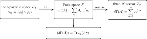
The lift $d\Gamma$ preserves the one-particle matrix information while extending the operator across all Fock sectors. On the $N$-particle sector it becomes the additive slot sum, and its mean value is determined by the one-body density matrix $\gamma$.

Hermiticity

Taking the adjoint gives

$$\begin{aligned} \widehat A^\dagger &= \sum_{i,j} A_{ij}^* a_j^\dagger a_i, \\ &= \sum_{i,j} A_{ji}^* a_i^\dagger a_j. \end{aligned}$$

Thus

$$\widehat A^\dagger = d\Gamma(A^\dagger).$$

If $A$ is Hermitian,

$$A_{ij} = A_{ji}^*,$$

and $\widehat A$ is Hermitian on the corresponding domain.

An off-diagonal bilinear $a_i^\dagger a_j$ is not Hermitian by itself for $i\ne j$. A Hermitian observable contains the conjugate transfer:

$$A_{ij}a_i^\dagger a_j + A_{ij}^*a_j^\dagger a_i.$$

Action Across Fock Sectors

The lift acts on every fixed-number sector:

$$\mathcal F = \bigoplus_{N=0}^{\infty} \mathcal F_N.$$

On the vacuum,

$$\widehat A\lvert0\rangle = 0.$$

On the one-particle sector, $\widehat A$ acts exactly as $A$. On the $N$-particle sector,

$$\left. \widehat A \right|_{\mathcal F_N} = \sum_{\alpha=1}^{N} A^{(\alpha)}.$$

Because each bilinear contains one creation and one annihilation operator,

$$[N,\widehat A] = 0.$$

A one-body operator may change mode occupations, spin projections, bands, or species labels while preserving total particle number.

The Identity Lifts to Number

For the one-particle identity,

$$I_{\mathcal H_1} = \sum_i \lvert\varphi_i\rangle \langle\varphi_i\rvert.$$

Its lift is

$$d\Gamma(I_{\mathcal H_1}) = \sum_i a_i^\dagger a_i = N.$$

This is a useful normalization check. On the fixed-$N$ sector, applying the one-particle identity to each particle adds $N$ copies of one, not one copy.

Zero-, One-, and Two-Body Structure

Operator degree should be classified by how many particles a term acts on, not only by the number of ladder symbols visible after a change of variables.

Structure	Typical form	Meaning
zero-body	$E_0 I$	constant energy or normalization offset
linear source	$\eta_i a_i^\dagger+\eta_i^*a_i$	creates or removes one particle; not an additive one-body lift
one-body	$A_{ij}a_i^\dagger a_j$	acts on one particle at a time and conserves number
pairing quadratic	$\Delta_{ij}a_i^\dagger a_j^\dagger+\text{h.c.}$	quadratic but number nonconserving; not $d\Gamma(A)$
two-body	$V_{ij;kl}a_i^\dagger a_j^\dagger a_l a_k$	acts on particle pairs

Calling every quadratic expression a one-body operator hides the distinction between number-conserving lifts and pairing or source terms.

Bosonic and Fermionic Action

For bosons and $i\ne j$,

$$\begin{aligned} a_i^\dagger a_j \lvert\ldots,n_i,\ldots,n_j,\ldots\rangle ={}& \sqrt{(n_i+1)n_j} \\ &\times \lvert\ldots,n_i+1,\ldots,n_j-1,\ldots\rangle. \end{aligned}$$

For fermions, the same bilinear transfers a particle only when $n_j=1$ and $n_i=0$. Its sign is fixed by the declared ordering of complete fermionic modes.

The lift formula has the same visible shape for both statistics, but its matrix elements do not. Bosonic Operators in Many-Body Models and Fermionic Operators in Many-Body Models own the detailed action rules.

Diagonal and Off-Diagonal Parts

Split

$$\widehat A = \sum_i A_{ii}n_i + \sum_{i\ne j} A_{ij}a_i^\dagger a_j.$$

The diagonal part is determined by mode occupations in the chosen basis. The off-diagonal part probes or generates one-body coherence.

Dropping the off-diagonal terms is justified only when:

• $A$ is diagonal in that basis;
• the off-diagonal matrix elements vanish by symmetry;
• or a stated approximation discards them.

A state diagonal in the occupation basis does not make an arbitrary one-body operator diagonal. State structure and operator structure are separate questions.

Basis Covariance

Let a new orthonormal basis be

$$\lvert\chi_\alpha\rangle = \sum_i \lvert\varphi_i\rangle U_{i\alpha},$$

with unitary $U$. The new annihilation operators are

$$b_\alpha = \sum_i U_{i\alpha}^* a_i,$$

and the matrix transforms as

$$A' = U^\dagger A U.$$

The Fock-space operator is invariant:

$$\sum_{\alpha,\beta} A'_{\alpha\beta} b_\alpha^\dagger b_\beta = \sum_{i,j} A_{ij}a_i^\dagger a_j.$$

Matrix elements and mode operators must be transformed together. Rotating only one of them changes the physical operator.

Diagonalizing a Hermitian One-Body Operator

If $A$ is Hermitian, choose eigenmodes

$$A\lvert\chi_\alpha\rangle = a_\alpha \lvert\chi_\alpha\rangle.$$

Then

$$\widehat A = \sum_\alpha a_\alpha b_\alpha^\dagger b_\alpha.$$

For a purely one-body Hamiltonian,

$$H_1 = d\Gamma(h),$$

this makes occupation-number states in the eigenmode basis many-body energy eigenstates:

$$E_{\boldsymbol n} = \sum_\alpha \epsilon_\alpha n_\alpha.$$

Diagonalizing $h$ does not solve an interacting Hamiltonian. The interaction transforms with the basis and generally remains quartic and nondiagonal.

Degeneracy and Basis Freedom

Within a degenerate eigenspace of $A$, the diagonal form does not select a unique basis. One may use that freedom to simplify another commuting symmetry, localize orbitals, preserve real structure, or reduce the complexity of interaction matrix elements.

If two one-particle Hermitian operators commute,

$$[A,B] = 0,$$

they admit a common eigenbasis under the usual spectral assumptions. Their lifts then commute as well. Degeneracy labels should be included in the complete mode index rather than suppressed when another operator acts inside the degenerate subspace.

Continuum Form

If $A_x$ is the position-space representation of the one-particle operator,

$$\widehat A = \int d^dx\, \psi^\dagger(x) A_x \psi(x).$$

Examples include:

$$\begin{aligned} N &= \int d^dx\, \psi^\dagger\psi, \\ T &= \int d^dx\, \psi^\dagger \left( -\frac{\hbar^2\nabla^2}{2m} \right) \psi, \\ U &= \int d^dx\, U(x)\psi^\dagger\psi. \end{aligned}$$

For differential operators, the domain and boundary conditions matter. Integrating by parts can move derivatives between fields only when the boundary term is controlled.

Field Operators in Many-Body Models owns the continuum field construction and regularization cautions. Real-Space Representation owns the normalized cell dictionary, finite-difference limit, and boundary implementation.

Lattice Form

On a lattice,

$$\widehat A = \sum_{i,j} A_{ij}a_i^\dagger a_j.$$

Representative structures are:

$$\begin{aligned} \text{onsite potential:} &\quad \sum_i U_i n_i, \\ \text{hopping:} &\quad \sum_{i,j}t_{ij}a_i^\dagger a_j, \\ \text{polarization:} &\quad \sum_i q\mathbf R_i n_i. \end{aligned}$$

Hopping is one-body even though it couples two sites. It transfers one particle at a time. An intersite density product $n_i n_j$ is two-body because it couples simultaneous occupations.

The current generated by hopping is developed in Density Operators and Current Operators. The Tight-Binding Model owns the model-level diagonalization, boundary conditions, and band interpretation of these hopping matrices.

Complete Internal Labels

For orbital or site label $i$ and internal label $\alpha$,

$$\widehat A = \sum_{i,j} \sum_{\alpha,\beta} A_{i\alpha,j\beta} a_{i\alpha}^\dagger a_{j\beta}.$$

The matrix can contain:

• spin rotations and Zeeman coupling;
• spin-orbit-coupled hopping;
• orbital hybridization;
• interband transitions;
• coherent species conversion;
• sublattice mixing.

For spin-$1/2$, a local spin operator is

$$S_i^a = \frac{\hbar}{2} \sum_{\alpha,\beta} c_{i\alpha}^\dagger (\sigma^a)_{\alpha\beta} c_{i\beta}.$$

It is one-body and preserves total particle number, though it can change $N_\uparrow$ and $N_\downarrow$ separately.

External Probes

A classical probe that couples to a one-particle observable produces

$$H_{\mathrm{probe}}(t) = -f(t)\widehat A.$$

Examples include:

• an electric field coupled to dipole or polarization;
• a magnetic field coupled to spin or magnetic moment;
• a scalar potential coupled to density;
• a vector potential coupled through the current and diamagnetic terms;
• a laser or radio-frequency field coupling internal states.

The perturbation is one-body even when the response is strongly many-body. Interactions change the state, spectrum, matrix elements, and response function.

One-Body Reduced Density Matrix

For a many-body density operator $\rho_{\mathrm{MB}}$, define

$$\gamma_{ij} = \operatorname{Tr}_{\mathcal F} \left( \rho_{\mathrm{MB}} a_j^\dagger a_i \right).$$

Then

$$\gamma^\dagger = \gamma, \qquad \gamma \geq 0,$$

and

$$\operatorname{Tr}_{\mathcal H_1}\gamma = \langle N\rangle.$$

For a fixed-$N$ state, the trace-one reduced state is

$$\rho^{(1)} = \frac{\gamma}{N}.$$

The unnormalized convention is often more convenient in many-body theory because its eigenvalues are mean occupations.

Expectation Values From the One-Body Matrix

Every one-body expectation is determined by $\gamma$:

$$\begin{aligned} \langle\widehat A\rangle &= \sum_{i,j} A_{ij} \gamma_{ji}, \\ &= \operatorname{Tr}_{\mathcal H_1} \left( A\gamma \right). \end{aligned}$$

If $A$ is diagonal,

$$\langle\widehat A\rangle = \sum_i A_i \langle n_i\rangle.$$

If $A$ is not diagonal, off-diagonal coherences $\gamma_{ji}$ are required.

Two different many-body states can have the same $\gamma$ and therefore agree on every one-body expectation while differing in pair correlations, entanglement, or higher moments. One-body data are complete for one-body observables, not for the full many-body state.

Natural-Orbital Basis

Diagonalizing

$$\gamma \lvert\chi_\alpha^{\mathrm{nat}}\rangle = \nu_\alpha \lvert\chi_\alpha^{\mathrm{nat}}\rangle$$

defines natural orbitals and natural occupations. In that basis,

$$\gamma_{\alpha\beta} = \nu_\alpha\delta_{\alpha\beta}.$$

This basis diagonalizes the state’s one-body coherence, not necessarily the Hamiltonian or the interaction. Natural occupations and their interpretation are developed canonically in Occupation Numbers. Off-Diagonal Long-Range Order owns the thermodynamic scaling of natural occupations for bosonic condensation and the Pauli obstruction for fermions.

Transition One-Body Density Matrix

For initial and final many-body states, define

$$\gamma_{ij}^{fi} = \langle\Psi_f\vert a_j^\dagger a_i \vert\Psi_i\rangle.$$

Then

$$\langle\Psi_f\vert \widehat A \vert\Psi_i\rangle = \sum_{i,j} A_{ij} \gamma_{ji}^{fi}.$$

This factorization separates the probe or operator matrix $A_{ij}$ from the many-body transition information.

Transition one-body densities appear in spectroscopy, response theory, quantum chemistry, and nuclear structure. They are not ordinary density operators: for $f\ne i$, they need not be positive or Hermitian.

Connectivity of Basis States

A one-body bilinear changes at most one occupied mode into one other mode.

For fermionic Slater determinants, a one-body matrix element can be nonzero only when the determinants:

• are identical;
• or differ by one occupied spin-orbital replacement.

Determinants differing by two or more replacements require a two-body or higher operator at the basis-state level. Fermionic ordering still supplies the sign.

For bosonic number states, a bilinear changes one occupation down by one and another up by one. This sparse connectivity is central in exact diagonalization and configuration-interaction calculations.

Interacting eigenstates are superpositions of basis states, so their full transition matrix elements can connect complicated states even though every contributing bilinear has one-particle connectivity.

Algebra of Bilinears

For canonical bosonic or fermionic modes, ordinary commutators of number-conserving bilinears satisfy

$$\begin{aligned} [a_i^\dagger a_j,a_k^\dagger a_l] ={}& \delta_{jk}a_i^\dagger a_l \\ &- \delta_{il}a_k^\dagger a_j. \end{aligned}$$

Consequently,

$$[d\Gamma(A),d\Gamma(B)] = d\Gamma([A,B]).$$

The map $d\Gamma$ preserves the Lie algebra of one-particle operators. No statistics-dependent sign remains in the final bilinear commutator.

This identity is useful for:

• lifting symmetry generators;
• deriving equations of motion;
• checking conserved one-body quantities;
• constructing orbital rotations;
• recognizing closed algebras of collective bilinears.

Domain qualifications are required for unbounded continuum operators, but the matrix identity is exact in finite mode spaces.

Symmetries and Conserved One-Body Quantities

For a purely one-body Hamiltonian

$$H_1 = d\Gamma(h),$$

if

$$[h,A] = 0,$$

then

$$[H_1,\widehat A] = 0.$$

With interactions,

$$H = H_1+V,$$

one must also check

$$[V,\widehat A] = 0.$$

A symmetry of the one-particle Hamiltonian need not survive an interaction, boundary condition, external field, or truncation. Conversely, many interactions preserve total number, spin, momentum, or another lifted generator.

Closed Dynamics for a Quadratic Hamiltonian

Let

$$H_1 = \sum_{i,j} h_{ij}a_i^\dagger a_j.$$

The one-body density matrix evolves as

$$i\hbar \frac{d\gamma}{dt} = [h,\gamma].$$

This equation is closed: knowing $\gamma(0)$ and $h(t)$ determines every later one-body expectation for the quadratic, number-conserving system.

For a possibly time-dependent one-body observable,

$$\begin{aligned} \frac{d}{dt} \langle\widehat A\rangle ={}& \frac{i}{\hbar} \langle[H,\widehat A]\rangle \\ &+ \left\langle d\Gamma(\partial_t A) \right\rangle. \end{aligned}$$

When $H=H_1$, the commutator closes on another one-body operator:

$$[H_1,\widehat A] = d\Gamma([h,A]).$$

Interactions Open a Hierarchy

For

$$H = H_1+V,$$

with a two-body interaction $V$, the one-body equation has the structure

$$i\hbar \frac{d\gamma}{dt} = [h,\gamma] + \mathcal C[\Gamma^{(2)}],$$

where $\Gamma^{(2)}$ is a two-body reduced density matrix and $\mathcal C$ denotes the interaction contraction. Its index convention, sum rules, and contraction with pair interactions are developed in Two-Body Operators.

The dynamics of $\gamma$ are no longer closed. The two-body density evolves using three-body information, producing the BBGKY-type hierarchy. Mean-field theories close this hierarchy approximately by expressing higher correlations in terms of lower ones.

This is a precise reason interacting many-body dynamics cannot generally be reduced to evolving occupied one-particle orbitals.

Means Versus Fluctuations

For Hermitian $A$, the one-body density matrix determines $\langle\widehat A\rangle$, but generally not $\langle\widehat A^2\rangle$.

Introduce

$$\eta = \begin{cases} +1,&\text{bosons},\\ -1,&\text{fermions}. \end{cases}$$

Using

$$a_j a_k^\dagger = \delta_{jk} + \eta a_k^\dagger a_j,$$

one finds

$$\begin{aligned} \widehat A^2 ={}& \sum_{i,l} (A^2)_{il} a_i^\dagger a_l \\ &+ \eta \sum_{i,j,k,l} A_{ij}A_{kl} a_i^\dagger a_k^\dagger a_j a_l. \end{aligned}$$

The first term is one-body; the second contains two-body information. Therefore the variance

$$\operatorname{Var}(\widehat A) = \langle\widehat A^2\rangle - \langle\widehat A\rangle^2$$

usually requires a two-body reduced density matrix even though $\widehat A$ itself is one-body.

Extensivity and Spectral Bounds

Suppose the one-particle Hermitian operator satisfies

$$a_{\min}I \leq A \leq a_{\max}I.$$

On the fixed-$N$ sector,

$$N a_{\min}I \leq d\Gamma(A) \leq N a_{\max}I.$$

Thus additive one-body observables normally scale extensively with particle number. The intensive average per particle is

$$\frac{\widehat A}{N}$$

on a fixed nonzero-$N$ sector.

If particle number is unbounded, even a bounded nonzero $A$ can have an unbounded Fock-space lift because arbitrarily many particles can contribute.

Projection and Active-Space Truncation

Let $P_1$ project onto retained one-particle modes. The directly projected operator is

$$A_P = P_1 A P_1,$$

with lift

$$d\Gamma(A_P).$$

This is exact only for the projected model. If $A$ couples retained and discarded modes, the truncated operator omits those matrix elements. Convergence of the Hamiltonian does not automatically guarantee convergence of every observable.

When high-energy modes are eliminated dynamically, let $\mathcal P$ project onto the retained many-body model space and let $S$ generate the decoupling transformation. A consistent effective observable can be

$$\widehat A_{\mathrm{eff}} = \mathcal P e^S \widehat A e^{-S}\mathcal P.$$

Even if $\widehat A$ began as one-body, the transformed effective operator can acquire two-body and higher terms. Effective Hamiltonians and effective observables must be derived at the same level of approximation.

Mean-Field One-Body Operators

Hartree, Fock, Kohn–Sham, Bogoliubov, and other approximations often produce an effective one-body matrix

$$h_{\mathrm{eff}}[\gamma].$$

Its bilinear form does not make the original interacting Hamiltonian one-body. The effective coefficients may:

• depend on the state or density;
• require self-consistency;
• break a symmetry at the solution level;
• omit connected correlations;
• include double-counting subtraction constants;
• depend on frequency or energy in a more general self-energy description.

A mean-field decoupling is an approximation, not an operator identity.

Quasiparticle Caution

A Hamiltonian diagonal in quasiparticle occupations,

$$H_{\mathrm{qp}} = E_0 + \sum_\alpha E_\alpha \beta_\alpha^\dagger\beta_\alpha,$$

is one-body in the quasiparticle operators. Its expression in the original particle operators may include pairing terms, constants, and a nontrivial vacuum.

The phrase one-body must therefore identify the degrees of freedom. Bare particles, projected orbitals, collective modes, and Bogoliubov quasiparticles need not define the same operator grading.

Computational Construction

To build a one-body operator in a finite many-body basis:

1. declare the complete ordered one-particle mode list;
2. compute $A_{ij}$ in that exact mode basis;
3. verify $A_{ij}=A_{ji}^*$ for a Hermitian observable;
4. generate each nonzero transfer $a_i^\dagger a_j$;
5. apply bosonic square-root factors or fermionic parity signs;
6. keep the source and destination selection rules;
7. assemble symmetry blocks only after checking commutators;
8. compare a one-particle-sector matrix with the original matrix $A$;
9. verify $[N,\widehat A]=0$ numerically;
10. test basis covariance under a small unitary rotation.

Sparse connectivity makes one-body operators inexpensive to apply relative to generic two-body operators, but poor mode ordering or dense $A_{ij}$ can still dominate a calculation.

Common Mistakes

• Using matrix elements from one basis with ladder operators from another.
• Reversing the source and destination indices in $A_{ij}a_i^\dagger a_j$.
• Keeping only diagonal occupations for a nondiagonal observable.
• Calling hopping a two-body term because it connects two sites.
• Calling pairing a one-body lift because it is quadratic.
• Forgetting the Hermitian-conjugate transfer.
• Suppressing spin or orbital labels that the operator mixes.
• Assuming diagonalization of $h$ solves an interacting Hamiltonian.
• Treating natural orbitals as Hamiltonian eigenmodes.
• Assuming the one-body density matrix determines fluctuations.
• Inferring a full-state equality from agreement of all one-body expectations.
• Using a one-particle symmetry test without checking the interaction.
• Projecting the Hamiltonian and observable inconsistently.
• Calling a self-consistent mean-field matrix an exact microscopic one-body Hamiltonian.
• Forgetting that one-body is relative to a chosen particle or quasiparticle description.

Canonical Boundaries

This page owns:

• practical use of one-body operators in interacting many-body settings;
• expectation and transition matrix elements from one-body density matrices;
• bilinear commutator closure and one-body equations of motion;
• basis choice, diagonalization, truncation, and effective-operator cautions;
• the distinction among exact, projected, mean-field, and quasiparticle one-body forms.

Other pages own:

• the foundational lift and number-state action: One-Body Operators;
• the compact lookup formula: Second-Quantized One-Body Operator;
• occupation probabilities and natural occupations: Occupation Numbers;
• coordinate-space fields: Field Operators in Many-Body Models;
• densities and currents: Density Operators and Current Operators;
• genuine pair interactions: Two-Body Operators.

Summary

• A one-body operator is the additive lift $d\Gamma(A)=\sum_{ij}A_{ij}a_i^\dagger a_j$.
• The bilinear transfers one particle from source mode $j$ to destination mode $i$.
• Hermiticity, symmetries, and basis changes lift directly from one-particle matrices.
• A one-body Hamiltonian diagonalizes into independent mode occupations; interactions generally do not.
• Every one-body expectation is $\operatorname{Tr}(A\gamma)$.
• One-body transition matrices encode spectroscopy and sparse basis connectivity.
• Bilinears obey the same matrix commutator algebra for bosons and fermions.
• Interactions couple one-body dynamics to higher reduced density matrices.
• One-body means do not determine fluctuations or the full many-body state.
• Projection and mean-field reduction can turn exact one-body operators into approximate effective operators with induced many-body pieces.

Exercises

Exercise 1: Identity and number

Show that the one-particle identity lifts to the total number operator and explain its action on a fixed-$N$ sector.

Solution

In an orthonormal basis,

$$I_{\mathcal H_1} = \sum_i \lvert\varphi_i\rangle \langle\varphi_i\rvert.$$

Therefore

$$d\Gamma(I_{\mathcal H_1}) = \sum_i a_i^\dagger a_i = N.$$

On $\mathcal F_N$, the number operator has eigenvalue $N$, so

$$\left. d\Gamma(I_{\mathcal H_1}) \right|_{\mathcal F_N} = N I_{\mathcal F_N}.$$

This agrees with adding one identity contribution from each of the $N$ formal particle slots.

Exercise 2: Hermitian transfer operator

Let

$$A = t \lvert1\rangle\langle2\rvert + t^* \lvert2\rangle\langle1\rvert.$$

Lift $A$ to Fock space and verify Hermiticity.

Solution

The nonzero matrix elements are

$$A_{12}=t, \qquad A_{21}=t^*.$$

Thus

$$\widehat A = t a_1^\dagger a_2 + t^*a_2^\dagger a_1.$$

Taking the adjoint gives

$$\widehat A^\dagger = t^*a_2^\dagger a_1 + t a_1^\dagger a_2 = \widehat A.$$

The first term transfers a particle from mode $2$ to mode $1$, and the second transfers it back.

Exercise 3: Two-mode basis rotation

Let

$$A = \begin{pmatrix} \epsilon & t\\ t & \epsilon \end{pmatrix},$$

with real $t$. Use

$$b_\pm = \frac{a_1\pm a_2}{\sqrt2}$$

to diagonalize $\widehat A$.

Solution

The symmetric and antisymmetric one-particle vectors are eigenvectors with eigenvalues

$$a_+ = \epsilon+t, \qquad a_- = \epsilon-t.$$

Therefore

$$\widehat A = (\epsilon+t)b_+^\dagger b_+ + (\epsilon-t)b_-^\dagger b_-.$$

The result holds for bosons or fermions. Statistics changes the allowed occupations, not the one-particle diagonalization.

Exercise 4: Expectation from a one-body density matrix

For

$$A = \begin{pmatrix} 2 & i\\ -i & -1 \end{pmatrix}, \qquad \gamma = \begin{pmatrix} 3/4 & 1/4\\ 1/4 & 1/4 \end{pmatrix},$$

compute $\langle\widehat A\rangle$.

Solution

Use

$$\langle\widehat A\rangle = \operatorname{Tr}(A\gamma).$$

The diagonal contributions are

$$2\left(\frac34\right) + (-1)\left(\frac14\right) = \frac54.$$

The off-diagonal contribution is

$$i\left(\frac14\right) + (-i)\left(\frac14\right) = 0.$$

Hence

$$\langle\widehat A\rangle = \frac54.$$

The trace of $\gamma$ is one, so this example can represent a one-particle state or normalized one-body reduced state.

Exercise 5: Bilinear commutator

Starting from the canonical bosonic or fermionic algebra, show that

$$[a_i^\dagger a_j,a_k^\dagger a_l] = \delta_{jk}a_i^\dagger a_l - \delta_{il}a_k^\dagger a_j.$$

Solution

For bosons, commute $a_j$ through $a_k^\dagger$ and $a_l$ through $a_i^\dagger$. Quartic terms cancel between the two product orders.

For fermions, use

$$a_j a_k^\dagger = \delta_{jk} - a_k^\dagger a_j$$

and

$$a_l a_i^\dagger = \delta_{li} - a_i^\dagger a_l.$$

The two minus signs acquired in reordering the quartic term make those quartic terms cancel here as well. The remaining contractions give

$$\delta_{jk}a_i^\dagger a_l - \delta_{il}a_k^\dagger a_j.$$

Thus the ordinary commutator of even fermionic bilinears has the same form as the bosonic result.

Exercise 6: Slater-determinant connectivity

Explain why a one-body operator has zero matrix element between two orthonormal Slater determinants that differ in two occupied spin-orbitals.

Solution

Each term

$$a_i^\dagger a_j$$

removes at most one occupied spin-orbital $j$ and inserts at most one spin-orbital $i$. Acting on one determinant can therefore produce only:

• the same determinant when $i=j$ is occupied;
• a determinant differing by one replacement;
• or zero.

It cannot replace two occupied spin-orbitals. Orthogonality then makes the overlap with a determinant differing by two replacements vanish. A two-body operator can make two replacements.

Exercise 7: Closed one-body dynamics

Let

$$H_1 = d\Gamma(h).$$

Use the bilinear commutator algebra to derive

$$i\hbar\dot\gamma = [h,\gamma].$$

Solution

For

$$\gamma_{ij} = \langle a_j^\dagger a_i\rangle,$$

the Heisenberg equation gives

$$i\hbar \frac{d}{dt} \langle a_j^\dagger a_i\rangle = \left\langle [a_j^\dagger a_i,H_1] \right\rangle.$$

Using the bilinear commutator,

$$\begin{aligned} i\hbar\dot\gamma_{ij} ={}& \sum_k h_{ik}\gamma_{kj} \\ &- \sum_k \gamma_{ik}h_{kj}. \end{aligned}$$

Therefore

$$i\hbar\dot\gamma = h\gamma-\gamma h = [h,\gamma].$$

No higher reduced density matrix appears because the Hamiltonian is one-body.

Exercise 8: Spectral bound on a fixed-number sector

Suppose

$$a_{\min}I \leq A \leq a_{\max}I.$$

Show that on the $N$-particle sector,

$$N a_{\min}I \leq d\Gamma(A) \leq N a_{\max}I.$$

Solution

For each formal particle slot $\alpha$,

$$a_{\min}I \leq A^{(\alpha)} \leq a_{\max}I.$$

Add the $N$ operator inequalities:

$$N a_{\min}I \leq \sum_{\alpha=1}^{N} A^{(\alpha)} \leq N a_{\max}I.$$

On the fixed-$N$ sector,

$$d\Gamma(A) = \sum_{\alpha=1}^{N} A^{(\alpha)},$$

which proves the result. The bound applies to bosonic and fermionic sectors because it follows before imposing exchange symmetry.

References

• A. L. Fetter and J. D. Walecka, Quantum Theory of Many-Particle Systems, Dover (2003).
• J. W. Negele and H. Orland, Quantum Many-Particle Systems, Westview Press (1998).
• P. Ring and P. Schuck, The Nuclear Many-Body Problem, Springer (1980).
• J.-P. Blaizot and G. Ripka, Quantum Theory of Finite Systems, MIT Press (1986).
• P. Coleman, Introduction to Many-Body Physics, Cambridge University Press (2015).
• H. Bruus and K. Flensberg, Many-Body Quantum Theory in Condensed Matter Physics, Oxford University Press (2004).
• A. J. Coleman, “Structure of fermion density matrices,” Reviews of Modern Physics 35, 668–686 (1963), doi:10.1103/RevModPhys.35.668.
• A. Szabo and N. S. Ostlund, Modern Quantum Chemistry: Introduction to Advanced Electronic Structure Theory, Dover (1996).
• T. Helgaker, P. Jørgensen, and J. Olsen, Molecular Electronic-Structure Theory, Wiley (2000).