Momentum-Space Representation

Momentum space turns spatial translation structure into algebra on mode labels. A translation-invariant one-body kernel becomes diagonal in wave vector, while a translation-invariant interaction becomes a vertex that preserves the sum of incoming and outgoing momenta. On a lattice, the corresponding label is crystal momentum, defined only modulo a reciprocal-lattice vector.

The basic tradeoff is

$$\text{locality in real space} \quad\longleftrightarrow\quad \text{broad coupling in momentum space},$$

whereas convolution or translation invariance in real space becomes multiplication or a conservation delta in momentum space.

This page develops many-body Hamiltonians and Fock-space operators in momentum representation. One-particle amplitudes and their Born interpretation live in Momentum-Space Representation. Transform calculations live in Momentum Representation, and the site-wide transform signs are fixed in Fourier Transform Conventions. The complementary continuum-cell-lattice dictionary is developed in Real-Space Representation.

Conventions

Unless stated otherwise:

• space has dimension $d$;
• $\mathbf k$ is a wave vector and $\mathbf p=\hbar\mathbf k$ is mechanical momentum for a free continuum particle;
• $\mathcal V=L^d$ is a finite periodic volume;
• $N_s$ is the number of lattice unit cells or sites in a single-orbital model;
• $\alpha,\beta$ label spin, orbital, sublattice, or another internal degree of freedom;
• repeated internal labels are summed only when a sum is displayed or explicitly stated;
• $a_{\mathbf k\alpha}$ denotes a bosonic or fermionic annihilation operator;
• $\widetilde v(\mathbf q)$ is the Fourier transform of a pair potential;
• continuum integrations use

$$\int_{\mathbf k} \equiv \int \frac{d^dk}{(2\pi)^d}.$$

For bosons use commutators; for fermions use anticommutators. A compact bracket notation is

$$[A,B]_{\mp} \equiv AB\mp BA,$$

with the upper minus sign for bosons and the lower plus sign for fermions.

Canonical Scope

This page owns:

• finite-volume and continuum field-mode normalization;
• many-body kinetic and translation-invariant one-body Hamiltonians;
• total momentum in occupation-number language;
• interaction vertices and momentum-transfer variables;
• momentum-space density operators;
• lattice Fourier normalization and Brillouin-zone kinematics;
• crystal momentum, Brillouin zones, and Umklapp kinematics;
• boundary-condition and cutoff cautions in momentum calculations.

Other pages retain their canonical roles:

• abstract one-particle momentum wavefunctions: Momentum-Space Representation;
• Fourier analysis and distributions: Fourier Transform;
• translation generators and conservation: Translations and Momentum;
• reciprocal lattices and Bloch characters: Crystalline Symmetry Preview;
• tight-binding Hamiltonians, chain dispersions, and finite lattice boundaries: Tight-Binding Model;
• field-operator definitions and regularization: Field Operators in Many-Body Models;
• pair-matrix-element conventions and reduced-density-matrix contractions: Two-Body Operators.

Why Momentum Space Helps

Momentum representation is useful when the Hamiltonian or state has translation structure. It can:

• diagonalize free or translation-invariant one-body motion;
• expose total-momentum conservation at each interaction vertex;
• label symmetry blocks for exact diagonalization;
• separate center-of-mass and relative motion;
• make long-wavelength and Fermi-surface limits visible;
• convert spatial derivatives into powers of $\mathbf k$;
• turn real-space convolution kernels into momentum-space multiplication.

It is not always the best basis. Traps, open boundaries, disorder, impurities, and sharply local observables can be simpler in real space.

Periodic-Box Transform

In a cubic periodic box of volume $\mathcal V=L^d$,

$$\psi_\alpha(\mathbf r) = \frac1{\sqrt{\mathcal V}} \sum_{\mathbf k} e^{i\mathbf k\cdot\mathbf r} a_{\mathbf k\alpha}.$$

The inverse transform is

$$a_{\mathbf k\alpha} = \frac1{\sqrt{\mathcal V}} \int_{\mathcal V} d^dr\, e^{-i\mathbf k\cdot\mathbf r} \psi_\alpha(\mathbf r).$$

Periodic boundary conditions quantize the wave vectors:

$$\mathbf k = \frac{2\pi}{L} \mathbf n, \qquad \mathbf n\in\mathbb Z^d.$$

For a rectangular box, replace $2\pi n_\mu/L$ by $2\pi n_\mu/L_\mu$ in each direction.

Orthogonality and Completeness in the Box

The plane-wave modes satisfy

$$\int_{\mathcal V} d^dr\, e^{i(\mathbf k-\mathbf k')\cdot\mathbf r} = \mathcal V \delta_{\mathbf k,\mathbf k'}.$$

The periodic delta distribution is

$$\delta_{\mathcal V}(\mathbf r-\mathbf r') = \frac1{\mathcal V} \sum_{\mathbf k} e^{i\mathbf k\cdot(\mathbf r-\mathbf r')}.$$

It acts as the identity on functions compatible with the periodic box.

Preservation of the Canonical Algebra

If the equal-time field algebra is

$$[\psi_\alpha(\mathbf r), \psi_\beta^\dagger(\mathbf r')]_{\mp} = \delta_{\alpha\beta} \delta_{\mathcal V}(\mathbf r-\mathbf r'),$$

then the mode operators obey

$$[a_{\mathbf k\alpha}, a_{\mathbf k'\beta}^\dagger]_{\mp} = \delta_{\mathbf k,\mathbf k'} \delta_{\alpha\beta}.$$

All same-type mode brackets vanish. The Fourier transform is unitary on the retained one-particle space, so it preserves bosonic or fermionic statistics.

Continuum Transform

In infinite volume, use

$$\psi_\alpha(\mathbf r) = \int_{\mathbf k} e^{i\mathbf k\cdot\mathbf r} a_\alpha(\mathbf k),$$

with inverse

$$a_\alpha(\mathbf k) = \int d^dr\, e^{-i\mathbf k\cdot\mathbf r} \psi_\alpha(\mathbf r).$$

The continuum mode algebra is

$$[a_\alpha(\mathbf k), a_\beta^\dagger(\mathbf k')]_{\mp} = (2\pi)^d \delta_{\alpha\beta} \delta^{(d)}(\mathbf k-\mathbf k').$$

The mode operator $a_\alpha(\mathbf k)$ is distribution valued. It is not the same dimensionless object as the finite-box $a_{\mathbf k\alpha}$.

Box-to-Continuum Dictionary

The thermodynamic-limit replacements are

$$\frac1{\mathcal V} \sum_{\mathbf k} \longrightarrow \int_{\mathbf k},$$

and, schematically at the allowed box momenta,

$$a_\alpha(\mathbf k) \longleftrightarrow \sqrt{\mathcal V} a_{\mathbf k\alpha}.$$

Correspondingly,

$$(2\pi)^d \delta^{(d)}(\mathbf k-\mathbf k') \longleftrightarrow \mathcal V \delta_{\mathbf k,\mathbf k'}.$$

These replacements must be applied consistently to the integration measure, delta functions, operators, and interaction prefactors. Mixing one box convention with one continuum convention is a common source of missing powers of volume.

Particle Number in Momentum Space

The total number operator is basis invariant:

$$\widehat N = \sum_{\mathbf k,\alpha} a_{\mathbf k\alpha}^\dagger a_{\mathbf k\alpha}$$

in a finite box, or

$$\widehat N = \sum_\alpha \int_{\mathbf k} a_\alpha^\dagger(\mathbf k) a_\alpha(\mathbf k)$$

in the continuum convention above.

Individual occupations

$$n_{\mathbf k\alpha} = a_{\mathbf k\alpha}^\dagger a_{\mathbf k\alpha}$$

need not be conserved when interactions scatter particles between momenta.

Kinetic Energy Becomes Diagonal

For nonrelativistic particles,

$$T = \sum_\alpha \int d^dr\, \psi_\alpha^\dagger(\mathbf r) \left( -\frac{\hbar^2\nabla^2}{2m_\alpha} \right) \psi_\alpha(\mathbf r).$$

Since

$$-\nabla^2 e^{i\mathbf k\cdot\mathbf r} = k^2 e^{i\mathbf k\cdot\mathbf r},$$

orthogonality gives

$$T = \sum_{\mathbf k,\alpha} \varepsilon_\alpha(\mathbf k) a_{\mathbf k\alpha}^\dagger a_{\mathbf k\alpha},$$

where

$$\varepsilon_\alpha(\mathbf k) = \frac{\hbar^2k^2}{2m_\alpha}.$$

The diagonalization follows from translation invariance and the plane-wave eigenvalue of $-\nabla^2$.

General Translation-Invariant One-Body Kernel

Consider

$$\begin{aligned} H_1 ={}& \sum_{\alpha,\beta} \int d^dr\,d^dr'\, \psi_\alpha^\dagger(\mathbf r) \\ &\times h_{\alpha\beta}(\mathbf r-\mathbf r') \psi_\beta(\mathbf r'). \end{aligned}$$

The dependence only on $\mathbf r-\mathbf r'$ expresses continuous translation invariance. Fourier transformation gives

$$H_1 = \sum_{\mathbf k} \sum_{\alpha,\beta} a_{\mathbf k\alpha}^\dagger h_{\alpha\beta}(\mathbf k) a_{\mathbf k\beta},$$

where

$$h_{\alpha\beta}(\mathbf k) = \int d^dx\, e^{-i\mathbf k\cdot\mathbf x} h_{\alpha\beta}(\mathbf x).$$

Momentum is diagonal, but internal labels can still mix through the matrix $h(\mathbf k)$.

Bands and Internal Components

At each $\mathbf k$, diagonalize the Hermitian matrix

$$h(\mathbf k) u_n(\mathbf k) = \varepsilon_n(\mathbf k) u_n(\mathbf k).$$

Defining band operators

$$\gamma_{n\mathbf k} = \sum_\alpha u_{n\alpha}(\mathbf k)^* a_{\mathbf k\alpha}$$

gives

$$H_1 = \sum_{n,\mathbf k} \varepsilon_n(\mathbf k) \gamma_{n\mathbf k}^\dagger \gamma_{n\mathbf k}.$$

Fourier transformation and band diagonalization are separate steps. A lattice Fourier transform resolves translation sectors; a $\mathbf k$-dependent unitary resolves orbital or sublattice mixing inside each sector.

Total Momentum Operator

For a translation-invariant continuum model,

$$\mathbf P = \sum_{\mathbf k,\alpha} \hbar\mathbf k\, a_{\mathbf k\alpha}^\dagger a_{\mathbf k\alpha}.$$

It acts on ladder operators as

$$[\mathbf P,a_{\mathbf k\alpha}^\dagger] = \hbar\mathbf k\, a_{\mathbf k\alpha}^\dagger,$$

and

$$[\mathbf P,a_{\mathbf k\alpha}] = -\hbar\mathbf k\, a_{\mathbf k\alpha}.$$

Thus a Fock basis vector has total momentum

$$\mathbf P_{\boldsymbol n} = \sum_{\mathbf k,\alpha} \hbar\mathbf k\, n_{\mathbf k\alpha}.$$

Momentum Charge of an Operator String

For

$$M = a_{\mathbf k_1}^\dagger \cdots a_{\mathbf k_p}^\dagger a_{\mathbf q_s} \cdots a_{\mathbf q_1},$$

the commutator is

$$\begin{aligned} [\mathbf P,M] ={}& \hbar \left( \sum_{i=1}^{p}\mathbf k_i - \sum_{j=1}^{s}\mathbf q_j \right) M. \end{aligned}$$

The string preserves total momentum exactly when the created and annihilated wave-vector sums agree.

This is the momentum analogue of number-charge counting in Number Operators and Conserved Quantities.

Translation Symmetry and Momentum Blocks

If

$$[H,\mathbf P] = 0,$$

then the Hamiltonian is block diagonal in total-momentum sectors. A state initialized in one sector remains there under closed-system evolution.

The converse practical warning is important: writing operators with momentum labels does not guarantee momentum conservation. External traps, boundaries, disorder, drives, or inconsistent cutoffs can connect different total momenta.

The symmetry derivation belongs to Translation-Invariant Hamiltonians.

Translationally Invariant Pair Interaction

Let

$$\begin{aligned} H_{\mathrm{int}} ={}& \frac12 \sum_{\alpha,\beta} \int d^dr\,d^dr'\, \psi_\alpha^\dagger(\mathbf r) \psi_\beta^\dagger(\mathbf r') \\ &\times v_{\alpha\beta}(\mathbf r-\mathbf r') \psi_\beta(\mathbf r') \psi_\alpha(\mathbf r). \end{aligned}$$

Define

$$\widetilde v_{\alpha\beta}(\mathbf q) = \int d^dx\, e^{-i\mathbf q\cdot\mathbf x} v_{\alpha\beta}(\mathbf x).$$

The finite-box momentum-space form is

$$\begin{aligned} H_{\mathrm{int}} ={}& \frac1{2\mathcal V} \sum_{\substack{\mathbf k_1,\mathbf k_2,\\ \mathbf k_3,\mathbf k_4}} \sum_{\alpha,\beta} \delta_{\mathbf k_1+\mathbf k_2, \mathbf k_3+\mathbf k_4} \\ &\times \widetilde v_{\alpha\beta} (\mathbf k_1-\mathbf k_3) a_{\mathbf k_1\alpha}^\dagger a_{\mathbf k_2\beta}^\dagger a_{\mathbf k_4\beta} a_{\mathbf k_3\alpha}. \end{aligned}$$

Under this Fourier convention, $\widetilde v(\mathbf q)$ has units of energy times volume. The combination $\widetilde v(\mathbf q)/\mathcal V$ multiplying the dimensionless mode operators therefore has units of energy, as the Hamiltonian requires.

The Kronecker delta is the integral over the center-of-mass coordinate. It enforces equality of total incoming and outgoing momentum.

Momentum-Transfer Form

Set

$$\mathbf k_3=\mathbf k, \qquad \mathbf k_4=\mathbf k',$$

and define the transfer

$$\mathbf q = \mathbf k_1-\mathbf k.$$

Momentum conservation fixes the other outgoing wave vector to $\mathbf k'-\mathbf q$. Therefore

$$\begin{aligned} H_{\mathrm{int}} ={}& \frac1{2\mathcal V} \sum_{\mathbf k,\mathbf k',\mathbf q} \sum_{\alpha,\beta} \widetilde v_{\alpha\beta}(\mathbf q) \\ &\times a_{\mathbf k+\mathbf q,\alpha}^\dagger a_{\mathbf k'-\mathbf q,\beta}^\dagger a_{\mathbf k'\beta} a_{\mathbf k\alpha}. \end{aligned}$$

Every term visibly satisfies

$$(\mathbf k+\mathbf q) + (\mathbf k'-\mathbf q) = \mathbf k+\mathbf k'.$$

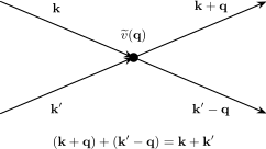
A translation-invariant two-body vertex transfers $\mathbf q$ from one line to the other. Individual momenta change, but the sum of the two outgoing wave vectors equals the sum of the two incoming wave vectors.

Ordered and Antisymmetrized Vertices

The displayed pair interaction uses ordered two-particle matrix elements and the prefactor $1/2$. For identical fermions one may instead use an antisymmetrized vertex,

$$\overline{\mathcal V}_{12;34} = \mathcal V_{12;34} - \mathcal V_{12;43},$$

with the prefactor $1/4$. Direct and exchange transfer channels are then packaged into $\overline{\mathcal V}$.

These prefactors must follow the coefficient convention, not visual inspection of the quartic string. The canonical comparison is in Two-Body Operators.

Contact Interaction

For

$$v(\mathbf r) = g\delta^{(d)}(\mathbf r),$$

the Fourier transform is independent of transfer:

$$\widetilde v(\mathbf q) = g.$$

Hence

$$\begin{aligned} H_{\mathrm{contact}} ={}& \frac{g}{2\mathcal V} \sum_{\mathbf k,\mathbf k',\mathbf q} a_{\mathbf k+\mathbf q}^\dagger a_{\mathbf k'-\mathbf q}^\dagger \\ &\times a_{\mathbf k'} a_{\mathbf k}. \end{aligned}$$

A constant momentum-space vertex does not mean that the particles do not scatter. It means that the idealized zero-range interaction has no transfer dependence before regularization.

In continuum dimensions where a contact interaction is ultraviolet sensitive, the bare $g$ depends on the regulator and must be matched to a physical scattering parameter.

Density Modes

Define the Fourier component of number density by

$$\rho_{\mathbf q} = \sum_{\mathbf k,\alpha} a_{\mathbf k+\mathbf q,\alpha}^\dagger a_{\mathbf k\alpha}.$$

With

$$n(\mathbf r) = \sum_\alpha \psi_\alpha^\dagger(\mathbf r) \psi_\alpha(\mathbf r),$$

the box Fourier pair is

$$\begin{aligned} n(\mathbf r) &= \frac1{\mathcal V} \sum_{\mathbf q} e^{i\mathbf q\cdot\mathbf r} \rho_{\mathbf q}, \\ \rho_{\mathbf q} &= \int_{\mathcal V}d^dr\, e^{-i\mathbf q\cdot\mathbf r} n(\mathbf r). \end{aligned}$$

It satisfies

$$\rho_{\mathbf q}^\dagger = \rho_{-\mathbf q},$$

and

$$\rho_{\mathbf0} = \widehat N.$$

The momentum carried by the density mode is

$$[\mathbf P,\rho_{\mathbf q}] = \hbar\mathbf q\, \rho_{\mathbf q}.$$

Thus $\rho_{\mathbf q}$ transfers wave vector $\mathbf q$ without changing particle number.

Interaction in Density Form

For a spin-independent pair potential,

$$H_{\mathrm{int}} = \frac1{2\mathcal V} \sum_{\mathbf q} \widetilde v(\mathbf q) :\rho_{\mathbf q} \rho_{-\mathbf q}:_0.$$

The empty-vacuum normal ordering removes the one-particle self-contraction and reproduces the pair interaction. Without the colons, a convention-dependent one-body self term appears.

Density modes are the natural operators for structure factors and density response, developed from the correlation side in Density Operators and Current Operators.

Momentum Distribution

For a state $\rho$, define

$$n_\alpha(\mathbf k) = \langle a_{\mathbf k\alpha}^\dagger a_{\mathbf k\alpha} \rangle.$$

Then

$$\langle\widehat N\rangle = \sum_{\mathbf k,\alpha} n_\alpha(\mathbf k).$$

For a translation-invariant state, the one-body momentum density matrix is diagonal up to symmetry-equivalent labels:

$$\langle a_{\mathbf k\alpha}^\dagger a_{\mathbf k'\beta} \rangle \propto \delta_{\mathbf k,\mathbf k'}.$$

Internal labels can remain off diagonal. Translation breaking at wave vector $\mathbf Q$ can instead produce coherence between $\mathbf k$ and $\mathbf k+\mathbf Q$.

Occupation Is Not Momentum Conservation

Momentum-conserving interactions generally satisfy

$$[H,\mathbf P] = 0$$

while

$$[H,n_{\mathbf k\alpha}] \neq 0.$$

Particles redistribute among modes while preserving the weighted sum $\sum\hbar\mathbf k n_{\mathbf k\alpha}$. Confusing conservation of total momentum with conservation of every mode occupation would incorrectly remove scattering.

External Potentials Mix Momenta

For a one-body external potential,

$$H_U = \sum_\alpha \int d^dr\, U(\mathbf r) \psi_\alpha^\dagger(\mathbf r) \psi_\alpha(\mathbf r),$$

define

$$\widetilde U(\mathbf q) = \int d^dr\, e^{-i\mathbf q\cdot\mathbf r} U(\mathbf r).$$

In a box,

$$H_U = \frac1{\mathcal V} \sum_{\mathbf k,\mathbf k',\alpha} \widetilde U(\mathbf k-\mathbf k') a_{\mathbf k\alpha}^\dagger a_{\mathbf k'\alpha}.$$

A constant potential contributes only at zero transfer and remains diagonal. A trap or impurity contains many Fourier components and mixes momenta. A periodic potential couples momenta separated by reciprocal-lattice vectors.

Center-of-Mass and Relative Momentum

For two particles, define

$$\mathbf K = \mathbf k_1+\mathbf k_2$$

and, for equal masses,

$$\mathbf k_{\mathrm{rel}} = \frac12 (\mathbf k_1-\mathbf k_2).$$

A translation-invariant pair interaction preserves $\mathbf K$ while changing relative momentum. The transfer variable $\mathbf q$ acts within a fixed center-of-mass sector.

For unequal masses, the mass-weighted relative coordinate and momentum should be used. The equal-mass half-difference is not universal.

Finite Volume and the Thermodynamic Limit

Periodic finite volume replaces integrals by discrete sums and Dirac deltas by Kronecker deltas. This is useful computationally and regulates infrared questions. The limit

$$L\to\infty$$

at fixed density makes the momentum grid dense:

$$\Delta k = \frac{2\pi}{L} \longrightarrow 0.$$

The ultraviolet range is a separate issue. Increasing $L$ at fixed grid spacing improves infrared resolution but does not automatically raise the momentum cutoff.

Lattice Fourier Transform

For a periodic Bravais lattice with $N_s$ cells at positions $\mathbf R_j$, define

$$a_{\mathbf k\alpha} = \frac1{\sqrt{N_s}} \sum_j e^{-i\mathbf k\cdot\mathbf R_j} a_{j\alpha},$$

and

$$a_{j\alpha} = \frac1{\sqrt{N_s}} \sum_{\mathbf k\in\mathrm{BZ}} e^{i\mathbf k\cdot\mathbf R_j} a_{\mathbf k\alpha}.$$

The allowed $\mathbf k$ values are the discrete translation characters compatible with the finite periodic lattice. The transform preserves the canonical mode algebra.

Translation-Invariant Hopping

Let

$$H_t = - \sum_{j,\boldsymbol\delta,\alpha} t_\alpha(\boldsymbol\delta) a_{j+\boldsymbol\delta,\alpha}^\dagger a_{j\alpha}.$$

Translation invariance means the hopping depends on displacement $\boldsymbol\delta$, not on $j$. Fourier transformation gives

$$H_t = \sum_{\mathbf k,\alpha} \varepsilon_\alpha(\mathbf k) a_{\mathbf k\alpha}^\dagger a_{\mathbf k\alpha},$$

with

$$\varepsilon_\alpha(\mathbf k) = - \sum_{\boldsymbol\delta} t_\alpha(\boldsymbol\delta) e^{-i\mathbf k\cdot\boldsymbol\delta}.$$

Hermiticity requires

$$t_\alpha(-\boldsymbol\delta) = t_\alpha(\boldsymbol\delta)^*,$$

which makes $\varepsilon_\alpha(\mathbf k)$ real.

Nearest-Neighbor Chain

For a one-dimensional chain with spacing $a$ and real nearest-neighbor hopping $t$,

$$H_t = -t \sum_j \left( a_{j+1}^\dagger a_j + a_j^\dagger a_{j+1} \right).$$

The dispersion is

$$\varepsilon(k) = -2t\cos(ka).$$

Momentum space diagonalizes the quadratic hopping, but the cosine remembers the finite lattice spacing and bounded Brillouin zone. The model-level derivation, open and twisted chains, bandwidth, effective mass, and multi-orbital extension live in Tight-Binding Model.

Multi-Orbital Unit Cells

With several orbitals or sublattices per cell,

$$H_0 = \sum_{\mathbf k} \sum_{\alpha,\beta} a_{\mathbf k\alpha}^\dagger h_{\alpha\beta}(\mathbf k) a_{\mathbf k\beta}.$$

The matrix $h(\mathbf k)$ is not generally diagonal. Its eigenvalues are bands, while its eigenvectors carry orbital composition.

Two common Fourier conventions use phases based on either the cell position $\mathbf R_j$ or the full orbital position $\mathbf R_j+\mathbf r_\alpha$. They differ by a $\mathbf k$-dependent diagonal unitary. Matrix entries and eigenvector phases change, while physical spectra and consistently computed observables do not.

Transforming an interaction from orbital operators to band operators inserts products of these eigenvectors as form factors. Consequently, even an onsite interaction that is momentum independent in the orbital basis generally acquires momentum and band dependence in the band basis.

Brillouin-Zone Preview

Reciprocal-lattice vectors satisfy

$$e^{i\mathbf G\cdot\mathbf R_j} = 1$$

for every Bravais-lattice vector $\mathbf R_j$. Therefore

$$\mathbf k \sim \mathbf k+\mathbf G.$$

A Brillouin zone chooses one representative from each equivalence class. In a one-dimensional lattice of spacing $a$, a standard first zone is

$$-\frac{\pi}{a} \le k < \frac{\pi}{a}.$$

The endpoints are equivalent. The Brillouin zone is not a hard wall in physical momentum; it is a fundamental domain for the crystal-momentum label.

Brillouin-Zone Integration

If the unit-cell volume is $v_c$, then

$$\operatorname{Vol}(\mathrm{BZ}) = \frac{(2\pi)^d}{v_c}.$$

In the large-lattice limit,

$$\frac1{N_s} \sum_{\mathbf k\in\mathrm{BZ}} \longrightarrow \frac{v_c}{(2\pi)^d} \int_{\mathrm{BZ}} d^dk.$$

This normalization is distinct from the continuum free-space integral when internal bands and unit-cell volumes are present.

Crystal-Momentum Conservation

Discrete translation symmetry conserves total crystal momentum only modulo a reciprocal vector:

$$\mathbf k_1+\mathbf k_2 - \mathbf k_3-\mathbf k_4 = \mathbf G.$$

Equivalently, the phase under every lattice translation is conserved. Folding all labels into one Brillouin zone can make a nonzero $\mathbf G$ appear in the representative equation even though the translation character is unchanged.

Crystal momentum should not be identified automatically with the total mechanical momentum of particles plus lattice.

Onsite Hubbard Interaction

For spin-$1/2$ fermions,

$$H_U = U \sum_j n_{j\uparrow}n_{j\downarrow}.$$

Its momentum-space form is

$$\begin{aligned} H_U ={}& \frac{U}{N_s} \sum_{\mathbf k,\mathbf k',\mathbf q} c_{\mathbf k+\mathbf q,\uparrow}^\dagger c_{\mathbf k'-\mathbf q,\downarrow}^\dagger \\ &\times c_{\mathbf k',\downarrow} c_{\mathbf k,\uparrow}, \end{aligned}$$

where all labels are understood modulo reciprocal vectors or accompanied by the appropriate crystal-momentum delta.

An onsite interaction is local in the site basis but couples every allowed transfer $\mathbf q$ in the momentum basis.

Bose–Hubbard Interaction

The Bose–Hubbard Model owns the full lattice model and its phases. This section owns only the momentum-space form of its onsite vertex.

For onsite bosons,

$$H_U^{(B)} = \frac U2 \sum_j n_j(n_j-1),$$

and

$$\begin{aligned} H_U^{(B)} ={}& \frac{U}{2N_s} \sum_{\mathbf k,\mathbf k',\mathbf q} b_{\mathbf k+\mathbf q}^\dagger b_{\mathbf k'-\mathbf q}^\dagger \\ &\times b_{\mathbf k'} b_{\mathbf k}. \end{aligned}$$

The factor $1/2$ avoids double counting identical boson pairs. The momentum-independent onsite vertex still generates nontrivial scattering and correlations.

Normal and Umklapp Processes

When all crystal momenta are represented in the first Brillouin zone:

• a normal process has $\mathbf G=\mathbf0$;
• an Umklapp process has $\mathbf G\neq\mathbf0$.

Umklapp is allowed by lattice translation symmetry because reciprocal vectors have trivial translation phase. Its effect on current or transport depends on the full model, occupations, dimensionality, and available phase space. The word does not by itself prove a finite resistivity.

Twisted Boundary Conditions

For a spatial twist $\boldsymbol\theta$,

$$\psi(\mathbf r+L\mathbf e_\mu) = e^{i\theta_\mu} \psi(\mathbf r).$$

The allowed components become

$$k_\mu = \frac{2\pi n_\mu+\theta_\mu}{L}.$$

Twists shift the finite-size momentum grid and are useful for flux insertion, stiffness, and boundary-condition averaging. A spatial antiperiodic boundary condition corresponds to $\theta_\mu=\pi$.

Do not confuse spatial twists with the bosonic or fermionic boundary conditions imposed in imaginary time at finite temperature.

Open Boundaries

With open boundaries, ordinary plane waves need not diagonalize the one-body Hamiltonian. Standing waves, sine transforms, or direct real-space methods may be natural. One may still Fourier transform data, but the resulting momentum labels are not exact translation quantum numbers.

Boundary terms also matter when deriving momentum conservation. A finite open sample can exchange momentum with its boundaries.

Momentum Cutoffs and Aliasing

A momentum-space calculation usually retains a finite set

$$\lvert\mathbf k\rvert \le \Lambda$$

or a finite grid. This can:

• modify contact interactions and require coupling renormalization;
• break rotational or translation symmetry if the cutoff is asymmetric;
• omit high-transfer virtual processes;
• produce aliasing in discrete transforms;
• induce effective many-body operators after modes are eliminated.

Every nonlinear product can generate wave vectors outside the retained grid. A numerical scheme must state whether those components are discarded, projected, or de-aliased.

Continuum and Lattice Comparison

Feature	Continuum	Periodic lattice
translation group	continuous	discrete Bravais lattice
label	mechanical wave vector for free particles	crystal momentum
equivalence	unique in reciprocal space	$\mathbf k\sim\mathbf k+\mathbf G$
domain	all $\mathbb R^d$ before cutoff	one Brillouin zone
kinetic term	often $\hbar^2k^2/(2m)$	band dispersion $\varepsilon_n(\mathbf k)$
conserved sum	exact momentum	crystal momentum modulo $\mathbf G$
local interaction prefactor	typically $1/\mathcal V$	typically $1/N_s$

The two descriptions approach one another only in a stated continuum limit near selected low-energy momenta.

Computational Workflow

For a momentum-space many-body calculation:

1. declare whether labels are $\mathbf p$ or $\mathbf k$;
2. state finite-volume, continuum, or lattice normalization;
3. derive the inverse transform and canonical algebra;
4. identify the actual translation symmetry and boundary conditions;
5. transform one-body and interaction terms with every volume factor visible;
6. distinguish ordered from antisymmetrized interaction coefficients;
7. enforce total momentum exactly or modulo reciprocal vectors as appropriate;
8. state the momentum grid, cutoff, and treatment of out-of-grid transfers;
9. verify Hermiticity and conserved charges numerically;
10. compare against a real-space calculation for small systems when possible.

Validation Checks

Useful checks include:

$$\sum_j e^{i(\mathbf k-\mathbf k')\cdot\mathbf R_j} = N_s \delta_{\mathbf k,\mathbf k'},$$ $$[a_{\mathbf k\alpha}, a_{\mathbf k'\beta}^\dagger]_{\mp} = \delta_{\mathbf k,\mathbf k'} \delta_{\alpha\beta},$$

and, for every nonzero interaction matrix element,

$$\mathbf k_1+\mathbf k_2 - \mathbf k_3-\mathbf k_4 = \begin{cases} \mathbf0,&\text{continuum},\\ \mathbf G,&\text{lattice}. \end{cases}$$

Also check the inverse transform, the one-particle dispersion, the trace of the one-body matrix, and box-versus-continuum normalization in finite-size tests.

Common Mistakes

• Mixing momentum $\mathbf p$ with wave vector $\mathbf k$ without $\mathbf p=\hbar\mathbf k$.
• Mixing box operators with continuum delta-normalized operators.
• Losing the factor $1/\mathcal V$ or $1/N_s$ in a quartic interaction.
• Assuming every momentum occupation is conserved because total momentum is conserved.
• Forgetting the exchange term when switching to antisymmetrized fermion vertices.
• Treating a constant contact vertex as an absence of scattering.
• Calling crystal momentum mechanical momentum.
• Requiring lattice momentum conservation with $\mathbf G=0$ only.
• Diagonalizing translation while forgetting orbital mixing inside $h(\mathbf k)$.
• Ignoring the Fourier phase convention for intra-cell orbital positions.
• Using plane waves as exact eigenmodes with open or trapped boundaries.
• Raising infrared resolution while leaving an ultraviolet cutoff unchanged, or vice versa.
• Assuming normal ordering alone makes a continuum contact interaction cutoff independent.

Quick Reference

Question	Formula or diagnostic
What is the box transform?	$\psi=\mathcal V^{-1/2}\sum_{\mathbf k}e^{i\mathbf k\cdot\mathbf r}a_{\mathbf k}$
How does the sum become an integral?	$\mathcal V^{-1}\sum_{\mathbf k}\to\int d^dk/(2\pi)^d$
Why is the kinetic term diagonal?	plane waves diagonalize translation-invariant derivatives
What does a density mode carry?	$[\mathbf P,\rho_{\mathbf q}]=\hbar\mathbf q\rho_{\mathbf q}$
What does a pair vertex conserve?	incoming and outgoing total momentum
What changes on a lattice?	momentum is defined modulo reciprocal vectors
What is the first Brillouin zone?	one representative per $\mathbf k\sim\mathbf k+\mathbf G$ class
What is Umklapp?	a symmetry-allowed process with nonzero reciprocal transfer $\mathbf G$
Does Fourier transformation diagonalize a multiband model?	only in $\mathbf k$; $h(\mathbf k)$ may still require diagonalization
Is a cutoff harmless?	no; it changes virtual processes and may require matching

Summary

• Finite-volume and continuum Fourier conventions use different operator and delta normalizations.
• Translation-invariant one-body kernels are diagonal in wave vector, up to internal-state mixing.
• Total continuum momentum is $\sum\hbar\mathbf k n_{\mathbf k\alpha}$.
• A translation-invariant pair interaction conserves total momentum at every vertex.
• The transfer variable $\mathbf q$ changes individual mode occupations while preserving their sum.
• Density modes $\rho_{\mathbf q}$ carry momentum $\hbar\mathbf q$ and organize interactions and response.
• Local real-space interactions become broad momentum-space quartic sums.
• Lattice Fourier transforms diagonalize translation sectors and produce band dispersions.
• Crystal momentum is defined modulo reciprocal-lattice vectors inside a Brillouin zone.
• Boundary conditions, orbital phase conventions, and cutoffs are part of the momentum-space model.

Exercises

Exercise 1: Canonical algebra in a periodic box

Starting from

$$a_{\mathbf k\alpha} = \frac1{\sqrt{\mathcal V}} \int_{\mathcal V}d^dr\, e^{-i\mathbf k\cdot\mathbf r} \psi_\alpha(\mathbf r),$$

derive the mode commutator or anticommutator.

Solution

Use the equal-time field algebra:

$$\begin{aligned} [a_{\mathbf k\alpha}, a_{\mathbf k'\beta}^\dagger]_{\mp} ={}& \frac1{\mathcal V} \int d^dr\,d^dr'\, e^{-i\mathbf k\cdot\mathbf r} e^{i\mathbf k'\cdot\mathbf r'} \\ &\times \delta_{\alpha\beta} \delta_{\mathcal V}(\mathbf r-\mathbf r'). \end{aligned}$$

The delta performs the $\mathbf r'$ integral, giving

$$\frac{\delta_{\alpha\beta}}{\mathcal V} \int_{\mathcal V}d^dr\, e^{i(\mathbf k'-\mathbf k)\cdot\mathbf r} = \delta_{\alpha\beta} \delta_{\mathbf k,\mathbf k'}.$$

Exercise 2: Diagonal kinetic energy

Transform

$$T = \int d^dr\, \psi^\dagger \left(-\frac{\hbar^2\nabla^2}{2m}\right) \psi$$

in a periodic box.

Solution

Insert the field expansions. The Laplacian acts on the annihilation-field plane wave:

$$-\nabla^2 e^{i\mathbf k'\cdot\mathbf r} = k'^2 e^{i\mathbf k'\cdot\mathbf r}.$$

Therefore

$$\begin{aligned} T ={}& \frac1{\mathcal V} \sum_{\mathbf k,\mathbf k'} \frac{\hbar^2k'^2}{2m} a_{\mathbf k}^\dagger a_{\mathbf k'} \\ &\times \int_{\mathcal V}d^dr\, e^{i(\mathbf k'-\mathbf k)\cdot\mathbf r}. \end{aligned}$$

Orthogonality sets $\mathbf k'=\mathbf k$, yielding

$$T = \sum_{\mathbf k} \frac{\hbar^2k^2}{2m} a_{\mathbf k}^\dagger a_{\mathbf k}.$$

Exercise 3: Interaction conservation delta

Show that the coordinate integral in a translation-invariant pair interaction produces

$$\delta_{\mathbf k_1+\mathbf k_2, \mathbf k_3+\mathbf k_4} \widetilde v(\mathbf k_1-\mathbf k_3).$$

Solution

The relevant integral is

$$\begin{aligned} I ={}& \int d^dr\,d^dr'\, e^{-i\mathbf k_1\cdot\mathbf r} e^{-i\mathbf k_2\cdot\mathbf r'} \\ &\times v(\mathbf r-\mathbf r') e^{i\mathbf k_4\cdot\mathbf r'} e^{i\mathbf k_3\cdot\mathbf r}. \end{aligned}$$

Set $\mathbf x=\mathbf r-\mathbf r'$ and keep $\mathbf r'$ as the center coordinate. The exponent becomes

$$-i(\mathbf k_1-\mathbf k_3)\cdot\mathbf x - i(\mathbf k_1+\mathbf k_2 -\mathbf k_3-\mathbf k_4) \cdot\mathbf r'.$$

The $\mathbf x$ integral gives $\widetilde v(\mathbf k_1-\mathbf k_3)$. The center-coordinate integral gives

$$\mathcal V \delta_{\mathbf k_1+\mathbf k_2, \mathbf k_3+\mathbf k_4}.$$

Combining this factor with the four field normalizations leaves the overall $1/\mathcal V$ vertex prefactor.

Exercise 4: Momentum carried by density

Using

$$\rho_{\mathbf q} = \sum_{\mathbf k,\alpha} a_{\mathbf k+\mathbf q,\alpha}^\dagger a_{\mathbf k\alpha},$$

show that $[\mathbf P,\rho_{\mathbf q}]=\hbar\mathbf q\rho_{\mathbf q}$.

Solution

Apply the commutator product rule:

$$\begin{aligned} [\mathbf P, a_{\mathbf k+\mathbf q,\alpha}^\dagger a_{\mathbf k\alpha}] ={}& \hbar(\mathbf k+\mathbf q) a_{\mathbf k+\mathbf q,\alpha}^\dagger a_{\mathbf k\alpha} \\ &- \hbar\mathbf k a_{\mathbf k+\mathbf q,\alpha}^\dagger a_{\mathbf k\alpha} \\ ={}& \hbar\mathbf q a_{\mathbf k+\mathbf q,\alpha}^\dagger a_{\mathbf k\alpha}. \end{aligned}$$

Summing over $\mathbf k,\alpha$ gives the result. The operator transfers momentum but preserves number.

Exercise 5: Nearest-neighbor lattice dispersion

Derive $\varepsilon(k)=-2t\cos(ka)$ for the periodic nearest-neighbor chain.

Solution

Use

$$a_j = \frac1{\sqrt{N_s}} \sum_k e^{ikaj}a_k.$$

Then

$$\sum_j a_{j+1}^\dagger a_j = \sum_k e^{-ika} a_k^\dagger a_k,$$

while the Hermitian conjugate gives $e^{ika}$. Therefore

$$\begin{aligned} H_t &= -t \sum_k \left( e^{-ika}+e^{ika} \right) a_k^\dagger a_k \\ &= \sum_k [-2t\cos(ka)] a_k^\dagger a_k. \end{aligned}$$

Exercise 6: Hubbard vertex

Transform $U\sum_jn_{j\uparrow}n_{j\downarrow}$ to momentum space and identify the conserved crystal-momentum combination.

Solution

Insert four lattice transforms. The site sum produces

$$\sum_j e^{i(-\mathbf k_1-\mathbf k_2 +\mathbf k_3+\mathbf k_4)\cdot\mathbf R_j} = N_s \delta^{(\mathbf G)}_{\mathbf k_1+\mathbf k_2, \mathbf k_3+\mathbf k_4}.$$

Three independent sums remain. Writing the transfer as $\mathbf q$ gives

$$\begin{aligned} H_U ={}& \frac U{N_s} \sum_{\mathbf k,\mathbf k',\mathbf q} c_{\mathbf k+\mathbf q,\uparrow}^\dagger c_{\mathbf k'-\mathbf q,\downarrow}^\dagger \\ &\times c_{\mathbf k',\downarrow} c_{\mathbf k,\uparrow}. \end{aligned}$$

The conserved combination is

$$\mathbf k_1+\mathbf k_2 - \mathbf k_3-\mathbf k_4 = \mathbf G.$$

Exercise 7: Brillouin-zone sum rule

Show that

$$\frac1{N_s} \sum_{\mathbf k\in\mathrm{BZ}} 1 = 1$$

is consistent with

$$\frac{v_c}{(2\pi)^d} \int_{\mathrm{BZ}}d^dk.$$

Solution

There are exactly $N_s$ allowed crystal momenta for each orbital in a periodic lattice of $N_s$ cells, so the discrete average equals one. In the thermodynamic limit,

$$\frac{v_c}{(2\pi)^d} \int_{\mathrm{BZ}}d^dk = \frac{v_c}{(2\pi)^d} \operatorname{Vol}(\mathrm{BZ}).$$

Using

$$\operatorname{Vol}(\mathrm{BZ}) = \frac{(2\pi)^d}{v_c}$$

gives one, matching the discrete normalization.

Exercise 8: Twisted momentum grid

For

$$\psi(x+L) = e^{i\theta} \psi(x),$$

derive the allowed $k$ values and recover periodic and antiperiodic cases.

Solution

A plane wave satisfies

$$e^{ik(x+L)} = e^{ikL}e^{ikx}.$$

The boundary condition requires

$$e^{ikL} = e^{i\theta}.$$

Therefore

$$kL = 2\pi n+\theta,$$

or

$$k_n = \frac{2\pi n+\theta}{L}.$$

Periodic boundaries have $\theta=0$. Spatial antiperiodic boundaries have $\theta=\pi$, shifting the grid by half a spacing.

References

1. A. L. Fetter and J. D. Walecka, Quantum Theory of Many-Particle Systems, Dover (2003).
2. J. W. Negele and H. Orland, Quantum Many-Particle Systems, Westview Press (1998).
3. G. D. Mahan, Many-Particle Physics, 3rd ed., Springer (2000).
4. P. Coleman, Introduction to Many-Body Physics, Cambridge University Press (2015).
5. A. Altland and B. Simons, Condensed Matter Field Theory, 2nd ed., Cambridge University Press (2010).
6. H. Bruus and K. Flensberg, Many-Body Quantum Theory in Condensed Matter Physics, Oxford University Press (2004).
7. N. W. Ashcroft and N. D. Mermin, Solid State Physics, Cengage Learning (1976).
8. E. Fradkin, Field Theories of Condensed Matter Physics, 2nd ed., Cambridge University Press (2013).
9. T. Giamarchi, Quantum Physics in One Dimension, Oxford University Press (2004).
10. L. Pitaevskii and S. Stringari, Bose–Einstein Condensation and Superfluidity, Oxford University Press (2016).