Two-Body Operator Applications

A number-conserving two-body operator acts on particle pairs. In an orthonormal one-particle basis, its standard Fock-space form is

$$\widehat V = \frac12 \sum_{i,j,k,l} V_{ij;kl} a_i^\dagger a_j^\dagger a_l a_k.$$

The operator annihilates an incoming pair in modes $k,l$ and creates an outgoing pair in modes $i,j$. The coefficient $V_{ij;kl}$ is a two-particle matrix element, and the prefactor depends on whether those matrix elements are unsymmetrized, symmetrized, antisymmetrized, or summed over a restricted index set.

The foundational equivalence with $\sum_{\alpha<\beta}v^{(\alpha\beta)}$ is derived in Two-Body Operators. This page is the many-body application guide: coefficient conventions, pair scattering, two-body reduced density matrices, basis transformations, contact and Coulomb interactions, lattice terms, symmetry tests, truncation, and computational checks.

Conventions

Unless stated otherwise:

• $\mathcal H_1$ is the one-particle Hilbert space;
• $\{\lvert\varphi_i\rangle\}$ is an orthonormal one-particle basis;
• each mode index includes every retained orbital, position, spin, species, band, or internal label;
• $a_i,a_i^\dagger$ are bosonic or fermionic mode operators;
• $\eta=+1$ for bosons and $\eta=-1$ for fermions;
• $v$ is a Hermitian, exchange-symmetric two-particle interaction;
• $V_{ij;kl}$ denotes matrix elements in the ordered product basis;
• sums run over the complete declared mode set unless restricted explicitly;
• $\Gamma^{(2)}$ is an unnormalized two-body reduced density matrix.

The semicolon in $V_{ij;kl}$ separates outgoing labels $i,j$ from incoming labels $k,l$. It is visual punctuation, not an additional tensor operation.

Canonical Scope

This page owns the practical use of number-conserving two-body operators in many-body models. It treats:

• unsymmetrized and statistics-adapted matrix-element conventions;
• bosonic occupation factors and fermionic signs;
• continuum, momentum-space, and lattice forms of two-body interactions;
• pair-density and two-body-density-matrix contractions;
• direct and exchange contributions;
• symmetry, truncation, and numerical validation.

Other pages retain their canonical roles:

• the foundational lift from first to second quantization: Two-Body Operators;
• complete many-particle Hamiltonian structure: Many-Particle Hamiltonians;
• statistics-specific ladder action: Bosonic Operators in Many-Body Models and Fermionic Operators in Many-Body Models;
• the complete many-body Fourier dictionary, one-body dispersions, density modes, and Brillouin-zone kinematics: Momentum-Space Representation;
• local density and current operators: Density Operators and Current Operators;
• phase structure of specific models, such as the Hubbard Model.

First-Quantized Pair Sum

On a fixed-$N$ sector, the same interaction is

$$\widehat V^{(N)} = \sum_{1\leq\alpha<\beta\leq N} v^{(\alpha\beta)}.$$

Every term acts on one unordered particle pair. If $v$ is symmetric under exchange of its two particle arguments, then

$$\widehat V^{(N)} = \frac12 \sum_{\alpha\neq\beta} v^{(\alpha\beta)}.$$

The number of contributing pairs is

$$\binom N2 = \frac{N(N-1)}2.$$

This counting explains both the factor $1/2$ and the absence of self-interaction for a one-particle state.

Ordered-Product Matrix Elements

Define

$$\begin{aligned} V_{ij;kl} ={}& \langle \varphi_i\otimes\varphi_j \vert v \vert \varphi_k\otimes\varphi_l \rangle. \end{aligned}$$

These are matrix elements on $\mathcal H_1\otimes\mathcal H_1$ before symmetrizing or antisymmetrizing the basis states. With this convention,

$$\widehat V = \frac12 \sum_{i,j,k,l} V_{ij;kl} a_i^\dagger a_j^\dagger a_l a_k.$$

Reading from right to left:

1. $a_k$ removes a particle from mode $k$;
2. $a_l$ removes a particle from mode $l$;
3. $a_j^\dagger$ creates a particle in mode $j$;
4. $a_i^\dagger$ creates a particle in mode $i$.

For fermions, this displayed order is part of the convention. Reordering a string and retaining the same coefficient without the corresponding sign changes the operator.

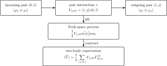
The ordered-product matrix element $V_{ij;kl}$ maps the incoming pair $(k,l)$ to the outgoing pair $(i,j)$. The Fock-space string preserves that order, while an expectation value contracts $V$ with the oppositely ordered indices of $\Gamma^{(2)}$.

Body Rank and Polynomial Degree

A number-conserving two-body interaction is quartic in ladder operators because it contains two creations and two annihilations. The two descriptions should not be conflated:

Structure	Representative form	Interpretation
one-body	$A_{ij}a_i^\dagger a_j$	acts additively on individual particles
two-body	$V_{ij;kl}a_i^\dagger a_j^\dagger a_l a_k$	acts on particle pairs
pairing quadratic	$\Delta_{ij}a_i^\dagger a_j^\dagger+\mathrm{h.c.}$	changes particle number by two; not a fixed-$N$ pair interaction
three-body	$W_{ijk;lmn}a_i^\dagger a_j^\dagger a_k^\dagger a_n a_m a_l$	acts on triples

A density product can hide this grading. For example, $n_i^2$ contains both a pair term and a one-body term for bosons. Normal ordering exposes the distinction.

Why the Prefactor Is One Half

The full sums over $i,j,k,l$ originate from a sum over ordered particle coordinates, while the physical interaction counts unordered pairs. The factor $1/2$ removes that duplicate counting.

The prefactor changes when the summation or coefficient convention changes. Three common choices are:

1. full index sums with unsymmetrized $V_{ij;kl}$ and prefactor $1/2$;
2. full sums with statistics-adapted coefficients and prefactor $1/4$;
3. restricted sums over unique pairs, with a prefactor determined by the restriction and pair-state normalization.

No prefactor is meaningful without its coefficient definition and summation domain.

Hermiticity

For a Hermitian two-particle operator $v$,

$$V_{ij;kl} = V_{kl;ij}^*.$$

Indeed,

$$\left( a_i^\dagger a_j^\dagger a_l a_k \right)^\dagger = a_k^\dagger a_l^\dagger a_j a_i.$$

Relabeling the incoming and outgoing index pairs then gives $\widehat V^\dagger=\widehat V$. In numerical work, the residual

$$V_{ij;kl}-V_{kl;ij}^*$$

is a direct diagnostic of integral-generation, storage, or convention errors.

Exchange Symmetry of the Interaction

Let $P_{12}$ exchange the two one-particle factors. A physical pair interaction for identical particles satisfies

$$[v,P_{12}]=0.$$

In the ordered product basis, this implies

$$V_{ij;kl} = V_{ji;lk}.$$

This identity exchanges both particles in the bra and ket. It does not generally imply $V_{ij;kl}=V_{ji;kl}$ or $V_{ij;kl}=V_{ij;lk}$ separately.

For a coordinate-diagonal symmetric potential $v(x,x')=v(x',x)$, the same relation follows by interchanging the integration variables.

Statistics-Adapted Coefficients

The ladder algebra projects the coefficient tensor onto the exchange sector appropriate to the particles. Define

$$W_{ij;kl}^{(\eta)} = V_{ij;kl} + \eta V_{ij;lk}.$$

For an exchange-symmetric interaction,

$$W_{ji;kl}^{(\eta)} = \eta W_{ij;kl}^{(\eta)}, \qquad W_{ij;lk}^{(\eta)} = \eta W_{ij;kl}^{(\eta)}.$$

The interaction may then be written

$$\widehat V = \frac14 \sum_{i,j,k,l} W_{ij;kl}^{(\eta)} a_i^\dagger a_j^\dagger a_l a_k.$$

For bosons, $W^{(+)}$ is symmetrized. For fermions, $W^{(-)}$ is antisymmetrized. This $W$ is not a normalized pair-basis matrix element; normalized states with coincident bosonic indices introduce additional square-root factors.

Fermionic Antisymmetrized Integrals

Fermionic many-body theory commonly writes

$$\langle ij\Vert kl\rangle = V_{ij;kl} - V_{ij;lk}.$$

Then

$$\widehat V = \frac14 \sum_{i,j,k,l} \langle ij\Vert kl\rangle c_i^\dagger c_j^\dagger c_l c_k.$$

The antisymmetrized integral obeys

$$\begin{aligned} \langle ji\Vert kl\rangle &= -\langle ij\Vert kl\rangle, \\ \langle ij\Vert lk\rangle &= -\langle ij\Vert kl\rangle. \end{aligned}$$

The $1/2$ and $1/4$ formulas represent the same operator. Using the $1/2$ prefactor with $\langle ij\Vert kl\rangle$ on a full index sum doubles the interaction.

Some quantum-chemistry texts order the last two annihilation indices differently. Always compare the integral definition and operator string together.

Bosonic Pair Matrix Elements

For bosons, only the part symmetric within each pair contributes. One may use

$$\langle ij\vert v\vert kl\rangle_+ = V_{ij;kl} + V_{ij;lk}$$

with the corresponding full-sum prefactor $1/4$. Alternatively, the unsymmetrized $V_{ij;kl}$ formula with prefactor $1/2$ is often simpler because the commuting ladder operators perform the symmetrization automatically.

When $i=j$ or $k=l$, a normalized bosonic pair state contains factorial normalization. Matrix elements between normalized pair states therefore should not be inserted into the unsymmetrized full-sum formula without converting conventions.

Action on Bosonic Number States

For four distinct modes,

$$\begin{aligned} &a_i^\dagger a_j^\dagger a_l a_k \lvert\ldots,n_i,\ldots,n_j,\ldots, n_k,\ldots,n_l,\ldots\rangle \\ &\quad= \sqrt{ (n_i+1)(n_j+1)n_k n_l } \\ &\qquad\quad\times \lvert\ldots,n_i+1,\ldots,n_j+1,\ldots, n_k-1,\ldots,n_l-1,\ldots\rangle. \end{aligned}$$

Coincident indices require sequential ladder action. Two important identities are

$$a_i^\dagger a_i^\dagger a_i a_i = n_i(n_i-1)$$

and

$$\begin{aligned} (a_i^\dagger)^2a_j^2 \lvert n_i,n_j\rangle ={}& \sqrt{(n_i+1)(n_i+2)} \\ &\times \sqrt{n_j(n_j-1)} \lvert n_i+2,n_j-2\rangle. \end{aligned}$$

The first counts ordered pairs in one mode; the Hamiltonian prefactor turns it into the unordered-pair count $n_i(n_i-1)/2$.

Action on Fermionic Number States

For fermions, a quartic term is nonzero only when:

• both required incoming modes are occupied;
• the outgoing modes are available after the annihilations;
• no repeated creation or annihilation index violates Pauli exclusion.

The sign is determined by the declared global mode ordering. It is safest to apply the operators from right to left with the same parity rule used for every fermionic basis state.

A two-body operator connects Slater determinants that differ by at most two occupied spin-orbital replacements. This is the origin of the double-excitation selection rule in configuration interaction. The value still includes direct, exchange, and ordering signs; connectivity alone does not determine the matrix element.

Diagonal Pair Counting

For different modes $i\neq j$,

$$a_i^\dagger a_j^\dagger a_j a_i = n_i n_j$$

for bosons or fermions. For one bosonic mode,

$$a_i^\dagger a_i^\dagger a_i a_i = n_i(n_i-1).$$

For one fermionic mode, the same quartic string vanishes because $(c_i^\dagger)^2=0$. Opposite spins on one lattice site are different modes, so their pair projector need not vanish.

These identities distinguish $n_i^2$ from pair counting:

$$n_i^2 = n_i(n_i-1)+n_i$$

for bosons. Replacing a pair interaction by $n_i^2$ adds a one-body term unless the Hamiltonian convention compensates for it.

Basis Covariance

Let a new orthonormal one-particle basis be

$$\lvert\chi_\alpha\rangle = \sum_i \lvert\varphi_i\rangle U_{i\alpha},$$

with unitary $U$. The new creation operators satisfy

$$b_\alpha^\dagger = \sum_i U_{i\alpha}a_i^\dagger.$$

The two-body tensor transforms as

$$\begin{aligned} V'_{\alpha\beta;\gamma\delta} ={}& \sum_{i,j,k,l} U_{i\alpha}^* U_{j\beta}^* V_{ij;kl} \\ &\times U_{k\gamma} U_{l\delta}. \end{aligned}$$

Using $V'$ with the $b$ operators gives the same many-body operator. A one-particle unitary rotation preserves body rank, Hermiticity, and exchange symmetry, but it need not preserve locality, density-density form, or sparsity.

A real-space onsite interaction, for example, generally becomes a momentum-scattering tensor after Fourier transformation.

Continuum Field Form

For a symmetric pair kernel $v(x,x')$,

$$\begin{aligned} \widehat V ={}& \frac12 \int dx\,dx'\, \psi^\dagger(x) \psi^\dagger(x') \\ &\times v(x,x') \psi(x') \psi(x). \end{aligned}$$

Here $x$ may include position and a discrete internal label. Expanding

$$\psi(x) = \sum_i \varphi_i(x)a_i$$

gives

$$\begin{aligned} V_{ij;kl} ={}& \int dx\,dx'\, \varphi_i^*(x) \varphi_j^*(x') \\ &\times v(x,x') \varphi_k(x) \varphi_l(x'). \end{aligned}$$

The Field Operators in Many-Body Models page owns distributional, dimensional, and cutoff details of the fields themselves.

Bosonic Contact Interaction

For a spinless bosonic low-energy model,

$$v(\mathbf r,\mathbf r') = g_B\delta^{(d)}(\mathbf r-\mathbf r').$$

Then

$$\widehat V_B = \frac{g_B}{2} \int d^dr\, \psi^\dagger \psi^\dagger \psi \psi,$$

with all fields evaluated at $\mathbf r$. Equivalently,

$$\widehat V_B = \frac{g_B}{2} \int d^dr\, {:}n^2(\mathbf r){:}.$$

This is an effective low-energy interaction. The relation between a bare cutoff-dependent coupling, a pseudopotential, and a measured scattering parameter depends on dimension and regularization. A formal delta function should not be treated as a universal microscopic potential.

Fermionic Contact Interaction

For two fermionic components, a standard intercomponent term is

$$\begin{aligned} \widehat V_F = g_F \int d^dr\, &\psi_\uparrow^\dagger \psi_\downarrow^\dagger \\ &\times \psi_\downarrow \psi_\uparrow. \end{aligned}$$

There is no factor $1/2$ because the ordered component pair $\uparrow,\downarrow$ is included once. Writing a symmetric sum over both component orders restores a compensating factor $1/2$.

A same-component zero-range $s$-wave term vanishes formally because

$$\psi_\sigma^\dagger(\mathbf r) \psi_\sigma^\dagger(\mathbf r) = 0.$$

This statement does not forbid finite-range or derivative interactions in odd partial waves.

Coulomb Interaction

For particles of charge magnitude $q$ in a medium with permittivity $\epsilon$,

$$v_C(\mathbf r,\mathbf r') = \frac{q^2} {4\pi\epsilon \lvert\mathbf r-\mathbf r'\rvert}.$$

The electron-electron term is

$$\begin{aligned} \widehat V_C ={}& \frac12 \sum_{\sigma,\sigma'} \int d^3r\,d^3r'\, \psi_\sigma^\dagger(\mathbf r) \psi_{\sigma'}^\dagger(\mathbf r') \\ &\times \frac{q^2} {4\pi\epsilon \lvert\mathbf r-\mathbf r'\rvert} \psi_{\sigma'}(\mathbf r') \psi_\sigma(\mathbf r). \end{aligned}$$

Spin is conserved by the interaction but still belongs to every mode label. In electronic-structure language, fixed-nucleus electron-nucleus attraction is one-body, whereas electron-electron repulsion is two-body.

Long-range Coulomb models also require boundary and neutrality conventions. In a periodic calculation, the treatment of the zero-momentum component, ionic background, and finite-size corrections is part of the model definition.

Lattice Density Interactions

A generic lattice density interaction can be written

$$\widehat V_{\mathrm{dd}} = \frac12 \sum_{i,j} U_{ij} a_i^\dagger a_j^\dagger a_j a_i,$$

where $i,j$ are complete lattice-mode labels. If $i\neq j$,

$$a_i^\dagger a_j^\dagger a_j a_i = n_i n_j.$$

When $U_{ij}=U_{ji}$ and only distinct sites are included,

$$\widehat V_{\mathrm{dd}} = \frac12 \sum_{i\neq j} U_{ij}n_i n_j.$$

If each unordered bond is listed once, the same interaction is

$$\widehat V_{\mathrm{dd}} = \sum_{\langle i,j\rangle} U_{ij}n_i n_j.$$

The summation symbol therefore carries normalization information.

Hubbard Onsite Interaction

For spin-$1/2$ fermions,

$$\widehat V_H = U\sum_r n_{r\uparrow}n_{r\downarrow}.$$

Using the fixed operator order,

$$n_{r\uparrow}n_{r\downarrow} = c_{r\uparrow}^\dagger c_{r\downarrow}^\dagger c_{r\downarrow} c_{r\uparrow}.$$

This is a two-body projector onto onsite double occupancy. Its local eigenvalue is one only on $\lvert\uparrow\downarrow\rangle_r$ and zero on the empty and singly occupied states.

The Hubbard Model owns the competition with hopping, symmetries, exact limits, and phase diagnostics.

Beyond Density-Density Terms

Two-body operators need not be diagonal in occupation number. Representative structures include:

$$c_{a\uparrow}^\dagger c_{b\downarrow}^\dagger c_{a\downarrow} c_{b\uparrow}$$

for spin exchange, and

$$c_{a\uparrow}^\dagger c_{a\downarrow}^\dagger c_{b\downarrow} c_{b\uparrow}$$

for pair hopping. Bosonic models can contain $(a_i^\dagger)^2a_j^2$, and projected interactions can generate density-assisted hopping.

Calling every quartic term a density interaction discards physically important scattering channels.

Momentum-Space Representation

For a translationally invariant continuum in volume $\Omega$, choose

$$\psi_\sigma(\mathbf r) = \frac{1}{\sqrt\Omega} \sum_{\mathbf k} e^{i\mathbf k\cdot\mathbf r} a_{\mathbf k\sigma}.$$

If $\widetilde v(\mathbf q)$ is the Fourier transform of $v(\mathbf r-\mathbf r')$, then

$$\begin{aligned} \widehat V ={}& \frac{1}{2\Omega} \sum_{\mathbf k,\mathbf k',\mathbf q} \sum_{\sigma,\sigma'} \widetilde v(\mathbf q) \\ &\times a_{\mathbf k+\mathbf q,\sigma}^\dagger a_{\mathbf k'-\mathbf q,\sigma'}^\dagger a_{\mathbf k',\sigma'} a_{\mathbf k,\sigma}. \end{aligned}$$

One particle gains momentum $\mathbf q$ while the other loses it. The total incoming and outgoing momenta agree term by term:

$$(\mathbf k+\mathbf q) + (\mathbf k'-\mathbf q) = \mathbf k+\mathbf k'.$$

For contact interactions, $\widetilde v(\mathbf q)$ is momentum independent within the effective theory. For the three-dimensional Coulomb kernel, it is proportional to $1/q^2$ away from $\mathbf q=0$.

On a lattice, crystal momentum is conserved modulo a reciprocal lattice vector, so Umklapp processes can occur.

This section records the interaction-specific formula. The finite-box and continuum normalization dictionary, kinetic terms, density modes, and lattice Fourier conventions are developed in Momentum-Space Representation.

Two-Body Reduced Density Matrix

For a many-body density operator $\rho_{\mathrm{MB}}$, define the unnormalized two-body reduced density matrix by

$$\Gamma_{ij;kl}^{(2)} = \operatorname{Tr} \left( \rho_{\mathrm{MB}} a_k^\dagger a_l^\dagger a_j a_i \right).$$

This convention mirrors

$$\gamma_{ij} = \operatorname{Tr} \left( \rho_{\mathrm{MB}}a_j^\dagger a_i \right)$$

for the one-body reduced density matrix. The two incoming indices appear first in $\Gamma^{(2)}$, while the creation indices appear after the semicolon.

Other communities reverse the pair order or divide by $N(N-1)$. A quoted two-body density matrix is incomplete unless its operator order and normalization are stated.

Off-Diagonal Long-Range Order uses these conventions to formulate Yang’s extensive-eigenvalue criterion for fermion-pair condensation. The present page retains ownership of the operator ordering, trace, contraction, and representability checks.

Expectation Values from the Two-Body Density Matrix

With the convention above,

$$\langle\widehat V\rangle = \frac12 \sum_{i,j,k,l} V_{ij;kl} \Gamma_{kl;ij}^{(2)}.$$

The reversed pair order is the matrix-trace contraction on the two-particle product space:

$$\langle\widehat V\rangle = \frac12 \operatorname{Tr}_{\mathcal H_1^{\otimes2}} \left( V\Gamma^{(2)} \right).$$

For antisymmetrized fermionic integrals,

$$\langle\widehat V\rangle = \frac14 \sum_{i,j,k,l} \langle ij\Vert kl\rangle \Gamma_{kl;ij}^{(2)}.$$

The one-body density matrix determines expectations of all one-body operators. The two-body density matrix is the additional object needed for all number-conserving pair interactions.

Exchange and Hermiticity of the Two-Body Density Matrix

The ladder algebra gives

$$\begin{aligned} \Gamma_{ji;kl}^{(2)} &= \eta\Gamma_{ij;kl}^{(2)}, \\ \Gamma_{ij;lk}^{(2)} &= \eta\Gamma_{ij;kl}^{(2)}, \\ \Gamma_{ij;kl}^{(2)*} &= \Gamma_{kl;ij}^{(2)}. \end{aligned}$$

For fermions, repeated indices within either pair vanish. For bosons, coincident indices encode same-mode pair occupation and need not vanish.

These identities are useful storage reductions and stringent numerical checks.

Trace and Contraction Sum Rules

The trace of the unnormalized two-body density matrix is

$$\sum_{i,j} \Gamma_{ij;ij}^{(2)} = \langle N(N-1)\rangle.$$

It counts ordered pairs. In a fixed-$N$ sector,

$$\sum_{i,j} \Gamma_{ij;ij}^{(2)} = N(N-1).$$

Partial contraction returns the one-body density matrix:

$$\sum_j \Gamma_{ij;kj}^{(2)} = (N-1)\gamma_{ik}$$

for fixed $N$. In a variable-particle-number state, one must retain the number-operator correlation; replacing $N$ by its mean generally does not give the exact contraction.

Positivity, exchange symmetry, trace, and contraction are necessary consistency checks, but they are not by themselves sufficient to guarantee that an arbitrary tensor is the two-body marginal of a valid many-fermion or many-boson state. This is the many-body representability problem.

Transition Two-Body Density Matrices

For initial and final many-body states, define

$$\Gamma_{ij;kl}^{fi} = \langle\Psi_f\vert a_k^\dagger a_l^\dagger a_j a_i \vert\Psi_i\rangle.$$

Then

$$\langle\Psi_f\vert \widehat V \vert\Psi_i\rangle = \frac12 \sum_{i,j,k,l} V_{ij;kl} \Gamma_{kl;ij}^{fi}.$$

Transition two-body densities encode pair-transfer and double-replacement amplitudes. They are not positive density operators and need not be Hermitian when $f\neq i$.

Pair Density and Pair Correlations

In the continuum, the diagonal pair density is

$$n^{(2)}(x,x') = \langle \psi^\dagger(x) \psi^\dagger(x') \psi(x') \psi(x) \rangle.$$

Its normalization is

$$\int dx\,dx'\, n^{(2)}(x,x') = \langle N(N-1)\rangle.$$

Where the one-body densities are nonzero, a normalized second-order coherence is

$$g^{(2)}(x,x') = \frac{n^{(2)}(x,x')} {n(x)n(x')}.$$

Here $n(x)=\langle\psi^\dagger(x)\psi(x)\rangle$ is the mean one-body density.

The interaction energy for a coordinate-diagonal pair kernel is

$$\langle\widehat V\rangle = \frac12 \int dx\,dx'\, v(x,x')n^{(2)}(x,x').$$

Mean density alone does not determine this energy in a correlated state. Pair avoidance, bunching, antibunching, and short-range correlation holes live in $n^{(2)}$ or the full $\Gamma^{(2)}$.

Slater Determinants and Direct Minus Exchange

For a fermionic Slater determinant, Wick factorization gives

$$\Gamma_{ij;kl}^{(2)} = \gamma_{ik}\gamma_{jl} - \gamma_{il}\gamma_{jk}.$$

In an occupied-orbital basis,

$$\langle\widehat V\rangle = \frac12 \sum_{p,q\in\mathrm{occ}} \left( V_{pq;pq} - V_{pq;qp} \right).$$

The first term is direct; the second is exchange. Exchange follows from fermionic antisymmetry even when $v$ itself is spin independent.

For opposite-spin orbitals, the exchange integral often vanishes because the spin functions are orthogonal. The direct interaction can remain nonzero.

An interacting exact state generally does not obey this factorization. The difference between its $\Gamma^{(2)}$ and the antisymmetrized product of $\gamma$ carries genuine two-particle correlation information.

What the Two-Body Density Matrix Does Not Determine

Together, $\gamma$ and $\Gamma^{(2)}$ determine every expectation value of number-conserving operators with body rank at most two. At fixed nonzero $N$, the contraction sum rule already recovers $\gamma$ from $\Gamma^{(2)}$. The two-body density matrix does not generally determine:

• the full many-body wavefunction or density operator;
• all three-body and higher observables;
• every entanglement property;
• real-time evolution under a two-body Hamiltonian without higher reduced densities.

The last point is important. The equation of motion for $\Gamma^{(2)}$ under a two-body Hamiltonian generally couples to a three-body reduced density matrix. This is the next level of the reduced-density hierarchy.

Symmetries and Conserved Quantities

Every term in the standard pair interaction has two creations and two annihilations, so

$$[N,\widehat V] = 0.$$

For another additive generator $Q=d\Gamma(q)$, the first-quantized criterion is

$$\left[ q\otimes I + I\otimes q, v \right] = 0.$$

When it holds,

$$[Q,\widehat V] = 0.$$

Examples include total momentum for a translationally invariant interaction and total spin for a spin-independent rotationally invariant interaction. A pair interaction can preserve the total generator while changing each particle or mode contribution separately.

Symmetry should be checked against the full coefficient tensor, boundary conditions, and truncation. A formally invariant continuum kernel can lose a symmetry after projection onto an asymmetric basis.

Vacuum Normal Ordering

The string

$$a_i^\dagger a_j^\dagger a_l a_k$$

is already normal ordered with respect to the empty Fock vacuum. Rewriting a non-normal-ordered density product can generate lower-body terms through commutators or anticommutators.

For example, bosons satisfy

$$n_i^2 = a_i^\dagger a_i^\dagger a_i a_i + n_i.$$

Thus $n_i^2$ and the normal-ordered pair operator differ by a one-body contribution.

Normal Ordering Relative to a Reference State

Normal ordering relative to a filled Slater determinant or correlated reference is a different operation. Contractions can decompose a two-body interaction schematically as

$$\widehat V = E_{\mathrm{ref}} + \widehat F_{\mathrm{ref}} + \widehat V_{\mathrm{res}},$$

where the three terms are zero-body, one-body, and residual two-body pieces relative to that reference.

This decomposition does not change the original physical body rank. It reorganizes the operator around a chosen state and underlies mean-field and many post-mean-field methods. The reference, contraction convention, and residual term must be stated together.

The explicit fermionic signs, Slater-determinant coefficients, correlated-reference cumulants, and normal-ordered rank truncations are developed in Normal Ordering in Many-Body QM.

Projection and Effective Interactions

Let $P_1$ project onto a retained one-particle subspace. Direct projection gives

$$v_P = (P_1\otimes P_1) v (P_1\otimes P_1),$$

followed by the ordinary two-body lift of $v_P$. This defines the interaction of the projected model.

It need not reproduce low-energy observables of the full model when discarded modes participate virtually. A dynamical decoupling transformation can renormalize the two-body coefficients and induce three-body and higher operators even if the microscopic Hamiltonian began with only pair interactions.

Dropping induced many-body terms is an approximation whose accuracy depends on scale separation, density, and the observable. Effective Hamiltonians in Many-Body Systems develops this issue through projected Hubbard and Anderson reductions.

Mean-Field Reduction Is Not an Identity

Hartree, Fock, Hartree–Fock, Bogoliubov, and related approximations replace part of a quartic interaction by state-dependent lower-degree operators. Schematically,

$$a_i^\dagger a_j^\dagger a_l a_k \longrightarrow \langle a_i^\dagger a_k\rangle a_j^\dagger a_l + \cdots.$$

The omitted terms and subtraction terms depend on the decoupling channel. A resulting one-body Hamiltonian is effective and state dependent; it does not prove that the original interaction was one-body.

Different decouplings emphasize density, exchange, pairing, or other order parameters. Comparing their energies requires consistent constants and double-counting corrections.

Computational Scaling and Structure

For $M$ one-particle modes, a dense unsymmetrized tensor has $M^4$ entries. Practical calculations exploit:

• Hermiticity and exchange symmetry;
• particle-number, spin, point-group, and momentum blocks;
• locality and finite interaction range;
• sparse determinant connectivity;
• low-rank, density-fitting, or Cholesky representations where justified;
• on-the-fly matrix-vector products instead of storing the full many-body matrix.

The formal $M^4$ count is not a universal runtime law. The useful complexity depends on the integral structure, basis, symmetry sectors, and numerical method.

Building a Two-Body Operator Numerically

A reliable finite-basis workflow is:

1. declare a complete ordered mode list;
2. state whether $V_{ij;kl}$ is unsymmetrized, symmetrized, or antisymmetrized;
3. state the full or restricted summation domain;
4. pair the coefficient convention with its correct prefactor;
5. verify $V_{ij;kl}=V_{kl;ij}^*$;
6. verify exchange identities appropriate to the convention;
7. apply annihilators and creators from right to left;
8. enforce bosonic factorials or fermionic parity signs;
9. compare the one-particle sector with zero interaction;
10. compare the two-particle sector with the direct first-quantized pair matrix;
11. check $[N,\widehat V]=0$ and any additional symmetry blocks;
12. test covariance under a small one-particle unitary rotation.

The two-particle-sector comparison is especially valuable: it tests prefactors, index order, exchange, and basis normalization before large Hilbert spaces obscure the error.

Common Mistakes

• Mixing the $1/2$ unsymmetrized convention with the $1/4$ antisymmetrized convention.
• Reversing $k,l$ in the coefficient while leaving $a_l a_k$ unchanged.
• Treating $V_{ij;kl}=V_{ji;lk}$ as symmetry under only one pair exchange.
• Inserting normalized pair-state matrix elements into an ordered-product full sum.
• Forgetting bosonic coincident-index factorials.
• Adding a fermionic exchange sign by hand after the ladder algebra already supplied it.
• Calling a pairing bilinear a number-conserving two-body interaction.
• Replacing $n(n-1)$ by $n^2$ without accounting for the one-body term.
• Using a same-component fermionic contact term without the derivative or finite-range structure needed to make it nonzero.
• Assuming a contact coupling is independent of cutoff and dimension.
• Ignoring charge neutrality and the zero mode in periodic Coulomb calculations.
• Inferring pair correlations from the mean density alone.
• Projecting the Hamiltonian but not the observables or induced many-body operators.

Quick Reference

Object	Convention used here
ordered-product integral	$V_{ij;kl}=\langle i,j\vert v\vert k,l\rangle$
unsymmetrized interaction	$\widehat V=\frac12\sum V_{ij;kl}a_i^\dagger a_j^\dagger a_l a_k$
fermionic antisymmetrized integral	$\langle ij\Vert kl\rangle=V_{ij;kl}-V_{ij;lk}$
antisymmetrized interaction	$\widehat V=\frac14\sum\langle ij\Vert kl\rangle c_i^\dagger c_j^\dagger c_l c_k$
two-body density matrix	$\Gamma_{ij;kl}^{(2)}=\langle a_k^\dagger a_l^\dagger a_j a_i\rangle$
interaction expectation	$\langle\widehat V\rangle=\frac12\sum V_{ij;kl}\Gamma_{kl;ij}^{(2)}$
fixed-$N$ trace	$\sum_{ij}\Gamma_{ij;ij}^{(2)}=N(N-1)$
bosonic onsite pair count	$(a_i^\dagger)^2a_i^2=n_i(n_i-1)$
Hubbard pair projector	$n_{r\uparrow}n_{r\downarrow}=c_{r\uparrow}^\dagger c_{r\downarrow}^\dagger c_{r\downarrow}c_{r\uparrow}$

Summary

• A number-conserving pair interaction is the lift of $\sum_{\alpha<\beta}v^{(\alpha\beta)}$.
• Ordered-product matrix elements use a full-sum prefactor $1/2$.
• Statistics-adapted full-sum coefficients use a prefactor $1/4$ in the convention defined here.
• Hermiticity exchanges incoming and outgoing pairs; particle exchange swaps both labels together.
• Bosonic ladder action supplies factorial enhancement, while fermionic action supplies exclusion and parity signs.
• Contact, Coulomb, Hubbard, exchange, and pair-hopping terms are realizations of the same operator structure.
• Two-body expectations contract the interaction tensor with $\Gamma^{(2)}$.
• Pair density contains information absent from mean density and the one-body reduced density matrix.
• Projection and reference normal ordering can generate effective lower- and higher-body terms.
• Two-particle-sector tests catch most convention errors before a large calculation begins.

Exercises

Exercise 1: Statistics-adapted prefactor

Let

$$W_{ij;kl}^{(\eta)} = V_{ij;kl} + \eta V_{ij;lk}.$$

Show that

$$\frac14 \sum_{i,j,k,l} W_{ij;kl}^{(\eta)} a_i^\dagger a_j^\dagger a_l a_k = \frac12 \sum_{i,j,k,l} V_{ij;kl} a_i^\dagger a_j^\dagger a_l a_k.$$

Solution

Write the contribution from the exchanged coefficient as

$$S = \sum_{i,j,k,l} \eta V_{ij;lk} a_i^\dagger a_j^\dagger a_l a_k.$$

Relabel $k\leftrightarrow l$:

$$S = \sum_{i,j,k,l} \eta V_{ij;kl} a_i^\dagger a_j^\dagger a_k a_l.$$

For bosons or fermions,

$$a_k a_l = \eta a_l a_k$$

when the coincident fermionic case is understood to vanish. Hence

$$S = \eta^2 \sum_{i,j,k,l} V_{ij;kl} a_i^\dagger a_j^\dagger a_l a_k.$$

Because $\eta^2=1$, the exchanged term equals the original term. The sum containing $W^{(\eta)}$ is therefore twice the unsymmetrized sum, and the prefactor changes from $1/2$ to $1/4$.

Exercise 2: Bosonic pair hopping

Evaluate

$$(a_1^\dagger)^2a_2^2 \lvert n_1,n_2\rangle.$$

State when the result vanishes.

Solution

Apply the two annihilators first:

$$a_2^2 \lvert n_1,n_2\rangle = \sqrt{n_2(n_2-1)} \lvert n_1,n_2-2\rangle.$$

Then create two particles in mode $1$:

$$\begin{aligned} (a_1^\dagger)^2a_2^2 \lvert n_1,n_2\rangle ={}& \sqrt{(n_1+1)(n_1+2)} \\ &\times \sqrt{n_2(n_2-1)} \lvert n_1+2,n_2-2\rangle. \end{aligned}$$

It vanishes for $n_2<2$. The total particle number is unchanged.

Exercise 3: Pair counting versus squared occupation

For one bosonic mode, prove

$$a^{\dagger2}a^2 = n(n-1)$$

and explain why $Un^2/2$ is not exactly the same onsite interaction as $Ua^{\dagger2}a^2/2$.

Solution

Acting on $\lvert n\rangle$ gives

$$a^2\lvert n\rangle = \sqrt{n(n-1)} \lvert n-2\rangle,$$

followed by

$$a^{\dagger2}a^2\lvert n\rangle = n(n-1)\lvert n\rangle.$$

The number states form a basis, so the operator identity follows. Since

$$n^2 = n(n-1)+n,$$

one has

$$\frac U2 n^2 = \frac U2 a^{\dagger2}a^2 + \frac U2 n.$$

The squared-occupation form contains an extra one-body term. At fixed total particle number its sum over sites may be a constant, but in a grand-canonical or spatially nonuniform setting it shifts one-particle energies or the chemical potential.

Exercise 4: Hubbard double occupancy

Show that

$$n_\uparrow n_\downarrow = c_\uparrow^\dagger c_\downarrow^\dagger c_\downarrow c_\uparrow,$$

and find its eigenvalue on the four local states.

Solution

Begin with

$$n_\uparrow n_\downarrow = c_\uparrow^\dagger c_\uparrow c_\downarrow^\dagger c_\downarrow.$$

Anticommuting $c_\uparrow$ through $c_\downarrow^\dagger$ gives one minus sign, and interchanging $c_\uparrow$ with $c_\downarrow$ gives a second:

$$n_\uparrow n_\downarrow = c_\uparrow^\dagger c_\downarrow^\dagger c_\downarrow c_\uparrow.$$

The eigenvalues are

$$\begin{array}{c|cccc} \text{state} &\lvert0\rangle &\lvert\uparrow\rangle &\lvert\downarrow\rangle &\lvert\uparrow\downarrow\rangle \\ \hline n_\uparrow n_\downarrow &0&0&0&1 \end{array}$$

so the Hubbard interaction assigns energy $U$ only to the doubly occupied state.

Exercise 5: Two-body density-matrix sum rules

For a fixed-$N$ state, prove

$$\sum_{i,j} \Gamma_{ij;ij}^{(2)} = N(N-1)$$

and

$$\sum_j \Gamma_{ij;kj}^{(2)} = (N-1)\gamma_{ik}.$$

Solution

For the trace,

$$\begin{aligned} \sum_{i,j} \Gamma_{ij;ij}^{(2)} &= \left\langle \sum_{i,j} a_i^\dagger a_j^\dagger a_j a_i \right\rangle \\ &= \langle N(N-1)\rangle. \end{aligned}$$

The operator counts an ordered choice of two distinct particles. On a fixed-$N$ sector, its eigenvalue is $N(N-1)$.

For the partial contraction,

$$\begin{aligned} \sum_j \Gamma_{ij;kj}^{(2)} &= \left\langle a_k^\dagger \left( \sum_j a_j^\dagger a_j \right) a_i \right\rangle \\ &= \langle a_k^\dagger N a_i\rangle. \end{aligned}$$

Acting on a fixed-$N$ state, $a_i$ first produces the $(N-1)$ sector. Therefore

$$\langle a_k^\dagger N a_i\rangle = (N-1) \langle a_k^\dagger a_i\rangle = (N-1)\gamma_{ik}.$$

Exercise 6: Direct and exchange energy

For a fermionic Slater determinant with occupied spin-orbitals $p,q$, use

$$\Gamma_{ij;kl}^{(2)} = \gamma_{ik}\gamma_{jl} - \gamma_{il}\gamma_{jk}$$

to derive its interaction energy.

Solution

In the occupied-orbital basis,

$$\gamma_{ij} = \delta_{ij}n_i, \qquad n_i\in\{0,1\}.$$

Insert the Slater two-body density into

$$\langle\widehat V\rangle = \frac12 \sum_{i,j,k,l} V_{ij;kl} \Gamma_{kl;ij}^{(2)}.$$

The first product of one-body densities sets $k=i$ and $l=j$; the second sets $k=j$ and $l=i$. Only occupied $i,j$ remain:

$$\langle\widehat V\rangle = \frac12 \sum_{p,q\in\mathrm{occ}} \left( V_{pq;pq} - V_{pq;qp} \right).$$

The two contributions are the direct and exchange integrals. For $p=q$, they cancel, excluding fermionic self-interaction.

Exercise 7: Momentum-space contact interaction

Take $\widetilde v(\mathbf q)=g$ in a periodic volume $\Omega$. Write the momentum-space interaction and identify the conserved quantity in every term.

Solution

Substitution gives

$$\begin{aligned} \widehat V ={}& \frac{g}{2\Omega} \sum_{\mathbf k,\mathbf k',\mathbf q} \sum_{\sigma,\sigma'} \\ &\times a_{\mathbf k+\mathbf q,\sigma}^\dagger a_{\mathbf k'-\mathbf q,\sigma'}^\dagger a_{\mathbf k',\sigma'} a_{\mathbf k,\sigma}. \end{aligned}$$

The incoming momentum is

$$\mathbf k+\mathbf k',$$

and the outgoing momentum is

$$(\mathbf k+\mathbf q) + (\mathbf k'-\mathbf q) = \mathbf k+\mathbf k'.$$

Total momentum is therefore conserved term by term. Particle number is also conserved because each term contains two creations and two annihilations.

Exercise 8: Additive symmetry test

Let $Q=d\Gamma(q)$ and suppose

$$\left[ q\otimes I + I\otimes q, v \right] = 0.$$

Explain why $[Q,\widehat V]=0$, and apply the statement to a translationally invariant pair potential.

Solution

On a fixed-$N$ sector,

$$Q^{(N)} = \sum_{\alpha=1}^N q^{(\alpha)}, \qquad \widehat V^{(N)} = \sum_{\alpha<\beta} v^{(\alpha\beta)}.$$

For a given pair $(\alpha,\beta)$, all $q^{(\gamma)}$ with $\gamma$ outside the pair commute with $v^{(\alpha\beta)}$. The remaining commutator is

$$\left[ q^{(\alpha)}+q^{(\beta)}, v^{(\alpha\beta)} \right],$$

which vanishes by the two-particle assumption. Summing over pairs gives

$$[Q^{(N)},\widehat V^{(N)}] = 0$$

in every sector, hence $[Q,\widehat V]=0$ on Fock space.

For translations, $q$ is one-particle momentum and a kernel $v(\mathbf r-\mathbf r')$ is invariant under simultaneous translation of both coordinates. Therefore total momentum commutes with the interaction, even though each particle can exchange momentum with the other.

References

1. A. L. Fetter and J. D. Walecka, Quantum Theory of Many-Particle Systems, Dover (2003).
2. J. W. Negele and H. Orland, Quantum Many-Particle Systems, Westview Press (1998).
3. P. Coleman, Introduction to Many-Body Physics, Cambridge University Press (2015).
4. A. Altland and B. Simons, Condensed Matter Field Theory, 2nd ed., Cambridge University Press (2010).
5. A. Szabo and N. S. Ostlund, Modern Quantum Chemistry, Dover (1996).
6. T. Helgaker, P. Jørgensen, and J. Olsen, Molecular Electronic-Structure Theory, Wiley (2000).
7. P. Ring and P. Schuck, The Nuclear Many-Body Problem, Springer (1980).
8. L. Pitaevskii and S. Stringari, Bose–Einstein Condensation and Superfluidity, Oxford University Press (2016).
9. A. J. Coleman, “Structure of Fermion Density Matrices,” Reviews of Modern Physics 35, 668–686 (1963), doi:10.1103/RevModPhys.35.668.
10. P.-O. Löwdin, “Quantum theory of many-particle systems. I. Physical interpretations by means of density matrices, natural spin-orbitals, and convergence problems in the method of configurational interaction,” Physical Review 97, 1474–1489 (1955), doi:10.1103/PhysRev.97.1474.
11. J. Hubbard, “Electron correlations in narrow energy bands,” Proceedings of the Royal Society A 276, 238–257 (1963), doi:10.1098/rspa.1963.0204.
12. E. Braaten and H.-W. Hammer, “Universality in few-body systems with large scattering length,” Physics Reports 428, 259–390 (2006), doi:10.1016/j.physrep.2006.03.001.