Quantum Optics

Quantum optics studies electromagnetic fields as quantum systems and asks how their states are prepared, transformed, coupled to matter, and measured. Its basic objects are not free-floating particles with unspecified wave functions. They are quantized field modes, their joint density operator, the physical devices that transform those modes, and detector models that turn the outgoing field into counts or currents.

That operational order matters. A statement such as “the beam contains one photon” is incomplete until the relevant spatial, temporal, spectral, and polarization mode has been declared. A statement such as “the light is coherent” is incomplete until the order of coherence and measured correlation function are stated. A claim of nonclassicality is incomplete until it names a criterion and accounts for loss, background, and detector resolution.

The compact organizing chain is

$$\begin{gathered} \text{mode definition} \\ \downarrow \\ \text{state preparation} \\ \downarrow \\ \text{transformation} \\ \downarrow \\ \text{measurement record} \\ \downarrow \\ \text{inferred property}. \end{gathered}$$

This chapter develops every stage of that chain. The present page is the map: it fixes notation, separates concepts that are often conflated, and identifies which later page owns each detailed derivation.

Canonical Scope

This chapter is the canonical home for quantum optics at the nonrelativistic and AMO level:

• quantum states of selected electromagnetic modes;
• photon-number, coherent, thermal, and squeezed light;
• passive and active optical transformations;
• direct, homodyne, heterodyne, and correlation measurements;
• optical coherence and nonclassicality criteria;
• cavity QED, the Jaynes–Cummings model, and practical input–output theory;
• nonlinear generation of quantum light.

Several foundations remain canonical elsewhere:

• The Quantum Harmonic Oscillator owns the oscillator spectrum and ladder-operator derivation.
• Coherent States owns their single-oscillator construction. Here they become states of specified optical modes and experimentally measured fields.
• Squeezed States: First Encounter owns the first oscillator treatment. This chapter develops generation, detection, loss, and optical applications.
• Fock Space owns the general occupation-number formalism. Here the occupied modes are electromagnetic.
• Light–Matter Interaction owns the progression from minimal coupling to few-level and dissipative AMO models.
• Quantum Optics as an Open-System Platform owns the master-equation, trajectory, and monitoring map.
• Wigner Functions own the general phase-space construction. Phase-Space Distributions compares the optical Wigner, Glauber–Sudarshan, and Husimi representations.

Full relativistic field quantization, photon propagators, renormalized QED, and high-energy scattering belong to the field-theory bridge. Quantizing a useful set of radiation modes is enough for much of laboratory quantum optics, but it is not a replacement for quantum electrodynamics.

Why Quantize Light?

Classical electrodynamics already explains interference, diffraction, polarization, propagation, and much of photodetection phenomenology. Quantum optics does not discard that success. It identifies experiments for which no classical stochastic electromagnetic field, combined with an adequate detector model, reproduces the observed statistics.

Three increasingly strong reasons for quantization should be distinguished.

Discrete energy exchange

A mode of angular frequency $\omega$ exchanges energy in units of $\hbar\omega$. Photoelectric and Compton phenomena established the importance of light quanta historically; see From Light Quanta to Photons. Discrete detector clicks alone, however, are not a universal proof that the incident field occupied a photon-number state. A classical field incident on a quantum, thresholded, or avalanche detector also produces discrete records. The statistics and correlations of those records carry the sharper information.

Vacuum and spontaneous processes

An excited atom coupled to an initially empty radiation continuum can emit a photon, become entangled with the emitted wave packet, and decay irreversibly after the continuum is eliminated. A simple semiclassical model with an exactly vanishing field does not initiate this process by itself. Field vacuum fluctuations and radiation reaction are representation-dependent parts of one physical quantum process, not separately measurable causes. The AMO derivation and its approximation hierarchy live on Spontaneous Emission.

Nonclassical statistics and correlations

Antibunching, sub-Poissonian counting, quadrature squeezing, Bell-inequality violations, and suitable phase-space negativities cannot be reproduced by a positive classical probability distribution over coherent fields. These are more discriminating tests than a low mean intensity or isolated clicks.

The boundary is therefore not “bright light is classical, dim light is quantum.” A weak coherent state is classical-like in the precise Glauber–Sudarshan sense, while a bright squeezed state can retain directly measurable nonclassical noise.

Modes as Harmonic Oscillators

The electromagnetic field has infinitely many degrees of freedom. A mode decomposition chooses an orthonormal set of solutions to the relevant classical wave problem, including boundary conditions and polarization. Each independent mode becomes a harmonic oscillator.

For discrete modes labelled by $\mu$,

$$[a_\mu,a_\nu^\dagger] = \delta_{\mu\nu}, \qquad [a_\mu,a_\nu] = 0,$$

and the free-field Hamiltonian is

$$H_{\mathrm{field}} = \sum_\mu \hbar\omega_\mu \left( a_\mu^\dagger a_\mu+\frac12 \right).$$

The number operator for mode $\mu$ is

$$N_\mu = a_\mu^\dagger a_\mu.$$

The same oscillator algebra appears in mechanics, but its physical normalization is fixed by electromagnetic energy. For orthonormal transverse mode functions $\mathbf f_\mu(\mathbf r)$ in a simple nondispersive vacuum geometry, one convenient positive-frequency field convention is

$$\mathbf E^{(+)}(\mathbf r,t) = i \sum_\mu \sqrt{ \frac{\hbar\omega_\mu}{2\epsilon_0} } \, \mathbf f_\mu(\mathbf r) a_\mu e^{-i\omega_\mu t}.$$

The negative-frequency part is $\mathbf E^{(-)}=(\mathbf E^{(+)})^\dagger$. Factors of volume migrate between $\mathbf f_\mu$ and the prefactor under other normalization conventions. In dielectric, dispersive, absorptive, waveguide, or quasinormal-mode settings, the energy normalization requires additional care. Copying a free-space “mode volume” formula into those settings can give the wrong coupling strength.

Discrete and continuous labels

A finite quantization box makes mode labels discrete and is often a calculation device. For a continuum, one instead uses operators such as $b(\omega)$ satisfying

$$[b(\omega),b^\dagger(\omega')] = \delta(\omega-\omega').$$

These operators are distributions, not dimensionless single-oscillator operators. A normalized temporal or spectral wave-packet mode is constructed from a square-integrable envelope:

$$\begin{aligned} A_f^\dagger &= \int d\omega\, f(\omega)b^\dagger(\omega), \\ \int d\omega\,|f(\omega)|^2 &= 1, \\ [A_f,A_f^\dagger] &= 1. \end{aligned}$$

The state $A_f^\dagger|0\rangle$ is one photon in the wave-packet mode $f$. Changing $f$ changes the state being asserted and the detector required to match it.

Mode choice is physical bookkeeping

Any unitary change of orthonormal mode basis,

$$c_j = \sum_\mu U_{j\mu}a_\mu, \qquad UU^\dagger = I,$$

preserves the bosonic commutators. Passive linear optics implements precisely such transformations between input and output modes. A mode basis may be plane-wave, cavity, Gaussian, time-bin, frequency-bin, polarization, or any other orthonormal basis suited to preparation and detection.

The total field is basis independent, but occupation statements are basis dependent. One photon in a superposition of two path modes is also one photon in a different output mode after the matching beam splitter. This is not ambiguity in the physics; it is the usual basis dependence of quantum state components.

Photons as Excitations of Modes

For one mode, the number states satisfy

$$\begin{aligned} N|n\rangle &= n|n\rangle, \\ a^\dagger|n\rangle &= \sqrt{n+1}\,|n+1\rangle, \\ a|n\rangle &= \sqrt n\,|n-1\rangle. \end{aligned}$$

A photon is one quantum of excitation of a specified electromagnetic mode. This definition immediately prevents several common category errors:

• a mode can be empty, singly occupied, or multiply occupied;
• one photon can occupy a spatially or temporally extended wave-packet mode;
• several orthogonal modes can overlap in ordinary space;
• a detector click is a measurement outcome, not automatically a nondestructive report of a pre-existing localized photon;
• indistinguishability means overlap in every mode degree of freedom relevant to the measurement, not merely equal central frequency.

The energy of a number state is

$$E_n = \hbar\omega \left( n+\frac12 \right).$$

Only energy differences are directly relevant for many isolated-mode experiments. The zero-point term becomes physically consequential through couplings, boundary dependence, fluctuations, and renormalized energy differences; treating the formal sum of all vacuum-mode energies as an ordinary finite observable is not justified.

Photon Number States develops the optical counting statistics, phase properties, source models, and nonclassicality of these states.

Occupation is not localization

Nonrelativistic particles admit a familiar position-space wavefunction. Photon localization is subtler because the electromagnetic field is relativistic, transverse, and gauge constrained. Laboratory quantum optics usually avoids an unnecessary photon-position operator. It predicts where and when a detector responds using field correlation functions and detector coupling.

For a one-photon wave packet $|1_f\rangle$, the detection amplitude in an idealized narrowband model is proportional to

$$\mathcal A(\mathbf r,t) \propto \langle 0| \mathbf E^{(+)}(\mathbf r,t) |1_f\rangle.$$

Its modulus squared helps determine a click-density envelope, but the full probability also depends on detector efficiency, response bandwidth, polarization sensitivity, and competing modes.

Classical-Like and Nonclassical Light

There is no single scalar “quantumness of light.” Different states expose different departures from a classical stochastic field description.

For one mode, define

$$\bar n = \langle N\rangle, \qquad (\Delta N)^2 = \langle N^2\rangle-\bar n^2,$$

and the zero-delay normalized second-order correlation

$$g^{(2)}(0) = \frac{ \langle a^\dagger a^\dagger aa\rangle }{ \langle a^\dagger a\rangle^2 } = \frac{ \langle N(N-1)\rangle }{ \bar n^2 },$$

provided $\bar n\ne0$.

The relation

$$g^{(2)}(0) = 1 + \frac{ (\Delta N)^2-\bar n }{ \bar n^2 }$$

connects coincidences to number fluctuations for a single stationary mode. It also shows why the mean photon number alone does not identify a state.

State	Number and correlation signature	Phase or quadrature character
number $	n\rangle$,$n\ge1$	exactly $n$; $g^{(2)}(0)=1-1/n$
coherent $	\alpha\rangle$	Poisson; $g^{(2)}(0)=1$
thermal	variance $=\bar n(\bar n+1)$; $g^{(2)}(0)=2$ for one mode	phase insensitive
squeezed vacuum	even photon numbers; $g^{(2)}(0)=3+1/\bar n$	one quadrature below vacuum

These ideal values assume one resolved mode, perfect stationarity where needed, and no background. Multimode averaging can drive thermal bunching toward one. Loss changes count rates and reconstructed states; detector jitter can wash out narrow correlation features.

Coherent light

A coherent state obeys

$$a|\alpha\rangle = \alpha|\alpha\rangle.$$

Its normally ordered field moments factorize, and passive linear optics maps products of coherent states to products of coherent states. These properties make coherent states the quantum states most closely associated with classical deterministic fields.

Real laser output is not literally a perfectly monochromatic pure coherent state over infinite time. Phase diffusion, amplitude noise, finite linewidth, technical noise, and the choice of temporal mode matter. “Laser light is coherent” is therefore a controlled approximation, not a complete density operator.

Coherent Light develops the multimode field, Poisson counting, all-order coherence, phase-reference problem, pure-loss stability, and realistic laser limits.

Thermal light

A single mode in thermal equilibrium has density operator

$$\rho_{\mathrm{th}} = \frac{1}{1+\bar n} \sum_{n=0}^{\infty} \left( \frac{\bar n}{1+\bar n} \right)^n |n\rangle\langle n|.$$

It has no preferred phase and exhibits bunching. Blackbody radiation is a multimode thermal field with frequency-dependent mean occupation

$$\bar n(\omega) = \frac{1}{ e^{\hbar\omega/(k_{\mathrm B}T)}-1 }.$$

Thermal statistics are not evidence of nonclassicality. Their correlations have a classical stochastic-wave representation.

Thermal Light develops the one-mode Gibbs state, geometric counts, bunching, multimode dilution, blackbody connection, and finite-resolution measurement caveats.

Squeezed light

With dimensionless quadratures

$$X = \frac{a+a^\dagger}{\sqrt2}, \qquad P = \frac{a-a^\dagger}{i\sqrt2},$$

one has

$$[X,P] = i, \qquad \Delta X\,\Delta P \ge \frac12.$$

Vacuum and coherent states have $(\Delta X)^2=(\Delta P)^2=1/2$. A squeezed state reduces one rotated quadrature below $1/2$ while increasing the conjugate variance. Squeezing does not evade the uncertainty relation; it redistributes noise.

Squeezed Light develops optical mode conventions, nonlinear generation, homodyne verification, decibel reporting, loss and phase-noise limits, and precision-measurement criteria.

A precise classicality criterion

The Glauber–Sudarshan representation writes

$$\rho = \int d^2\alpha\, P(\alpha) |\alpha\rangle\langle\alpha|.$$

If $P(\alpha)$ is an ordinary nonnegative probability density, all normally ordered moments can be interpreted as averages over classical complex field amplitudes. A state requiring a negative or more singular-than-probability $P$ distribution is called nonclassical in this optical sense.

Useful witnesses include:

• $g^{(2)}(0)<1$ for antibunching or sub-Poissonian statistics;
• quadrature variance below the vacuum level;
• negativity of an appropriate quasiprobability;
• entanglement or Bell violation across field modes.

These witnesses are not equivalent. Wigner negativity is sufficient for nonclassicality but not necessary: a squeezed Gaussian state has a nonnegative Wigner function while its $P$ representation is nonclassical. Conversely, thermal bunching with $g^{(2)}(0)>1$ is fully compatible with classical random waves.

The Operational Map

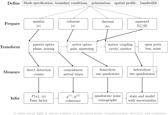
Quantum optics is an inference chain. The same source can give different records under different mode filters and detectors, and the same record can support different state models if loss or calibration is left unspecified.

The map separates four questions that should remain explicit in every calculation:

1. Which modes? Specify spatial profile, polarization, temporal or spectral envelope, normalization, and reference frame.
2. Which state? Give a ket only for a justified pure-state model; otherwise use a density operator over the retained modes.
3. Which transformation? Distinguish unitary mode mixing, active nonlinear evolution, matter coupling, and unobserved loss.
4. Which measurement? State the POVM or calibrated response connecting the outgoing field to counts, voltages, or reconstructed quadratures.

Skipping any stage hides assumptions inside a familiar formula.

Measurement of Light

Photodetection couples matter in a detector to the electromagnetic field. In the usual rotating-wave and broadband-detector approximation, absorption is sensitive to the positive-frequency field, and an ideal first-order count rate is proportional to

$$G^{(1)}(x,x) = \left\langle \mathbf E^{(-)}(x) \mathbin{\cdot} \mathbf E^{(+)}(x) \right\rangle,$$

where $x=(\mathbf r,t)$ includes the detector location and time. This normal ordering is not a typographical convention: an ideal absorber responds to annihilating an excitation rather than directly counting the symmetrized vacuum variance.

Direct photon counting

For one perfectly mode-matched field mode with number distribution $P_n$, an ideal number-resolving detector returns $n$ with probability $P_n$. A detector of quantum efficiency $\eta$ registers each incident excitation with probability $\eta$ in a simple independent-loss model:

$$p(m|n) = \binom{n}{m} \eta^m(1-\eta)^{n-m}.$$

An ideal on–off detector distinguishes zero registered counts from one or more. Its no-click POVM element is

$$\Pi_0 = \sum_{n=0}^{\infty} (1-\eta)^n |n\rangle\langle n|,$$

and $\Pi_{\mathrm{click}}=I-\Pi_0$. Dark counts, afterpulsing, dead time, timing jitter, saturation, and mode-dependent efficiency require extensions. Optical Photon Counting develops the calibrated detector response. The general measurement formalism belongs to POVMs; the conditional-record treatment belongs to open-system Photon Counting.

Homodyne detection

Balanced homodyne detection interferes the signal with a strong coherent local oscillator. The difference photocurrent isolates a signal quadrature whose angle is set by the local-oscillator phase:

$$X_\theta = \frac{ ae^{-i\theta} + a^\dagger e^{i\theta} }{ \sqrt2 }.$$

Sweeping $\theta$ samples quadrature distributions and can support state tomography. The local oscillator is also a mode selector: poor spatial, temporal, spectral, or polarization overlap appears as effective loss and admixed vacuum. Homodyne and Heterodyne Detection develops the receiver, calibration, selected modes, and quadrature POVM. The stochastic open-system account is developed on Homodyne Detection.

Heterodyne detection

Heterodyne detection accesses two conjugate quadratures in one measurement record by using a frequency-offset local oscillator or an equivalent dual-quadrature scheme. Simultaneous access comes with added vacuum noise. The resulting distribution is closely related to the Husimi $Q$ function, subject to gain and efficiency calibration. The optical implementation and coherent-state POVM are developed on Homodyne and Heterodyne Detection; the complex stochastic record belongs to Heterodyne Detection.

Measurement does not reveal a state without a model

No finite dataset uniquely announces its own Hilbert-space decomposition. State reconstruction requires:

• a calibrated detector response;
• an explicit retained-mode model;
• enough informationally complete settings;
• uncertainty propagation or likelihood intervals;
• checks for drift, loss, background, and model mismatch.

A negative reconstructed quasiprobability that disappears under plausible calibration variation is not a robust nonclassicality claim. Conversely, raw loss can hide nonclassicality without making the source state classical.

Correlations and Coherence

Classical first-order coherence describes field-amplitude interference. Quantum optical coherence extends the hierarchy to normally ordered multi-time, multi-position correlation functions.

For scalar notation, the first-order correlation is

$$G^{(1)}(1,2) = \left\langle E^{(-)}(1)E^{(+)}(2) \right\rangle,$$

with normalized form

$$g^{(1)}(1,2) = \frac{ G^{(1)}(1,2) }{ \sqrt{ G^{(1)}(1,1)G^{(1)}(2,2) } }.$$

$|g^{(1)}|$ controls fringe visibility under matched intensities. Its phase controls the fringe displacement. A field can have high first-order coherence without having coherent-state photon statistics.

The second-order correlation is

$$\begin{aligned} G^{(2)}_{12} \equiv{}& G^{(2)}(1,2) \\ ={}& \left\langle E_1^{(-)} E_2^{(-)} E_2^{(+)} E_1^{(+)} \right\rangle, \\ g^{(2)}(1,2) ={}& \frac{ G^{(2)}_{12} }{ I_1I_2 }, \\ I_j=G^{(1)}(j,j). \end{aligned}$$

It governs idealized coincidence rates. For a stationary source one often writes $g^{(2)}(\tau)$.

Bunching, Poisson statistics, and antibunching

For ideal single-mode examples:

$$\begin{array}{c|c} \text{state} & g^{(2)}(0) \\ \hline \text{coherent} & 1 \\ \text{thermal} & 2 \\ |1\rangle & 0 \end{array}$$

Thermal bunching was measured by Hanbury Brown and Twiss through intensity correlations. It has both classical random-wave and quantum photodetection descriptions and is not by itself a nonclassicality test. Antibunching, $g^{(2)}(0)<g^{(2)}(\tau)$ over an appropriate delay range, cannot arise from a stationary classical stochastic field under the standard assumptions. The stronger equal-time condition $g^{(2)}(0)<1$ is a common sub-Poissonian witness.

Experimental values must be tied to:

• bin width and detector timing response;
• background subtraction policy;
• normalization window;
• stationarity and blinking;
• number of collected spatial and spectral modes;
• detector dead time and cross-talk.

The formal value $g^{(2)}(0)=0$ for a perfect one-photon state does not mean that every real single-photon source yields a raw zero coincidence bin. Photon Antibunching develops the single-emitter mechanism, classical inequalities, measured dip models, and interpretation pitfalls.

Coherence is a hierarchy

Glauber coherence of order $n$ concerns factorization properties of $G^{(n)}$. Monochromaticity, narrow linewidth, first-order fringe visibility, Poissonian counts, and coherent-state purity are related in ideal models but are not synonyms. A trustworthy statement names the measured order and the space-time arguments.

Transforming Quantum Light

Optical devices are classified by what they do to mode operators and whether additional environmental modes must be included.

Passive linear optics

Lossless beam splitters, phase shifters, polarization rotations, and interferometers implement

$$\mathbf a_{\mathrm{out}} = U\mathbf a_{\mathrm{in}}, \qquad U^\dagger U = I.$$

They preserve commutators and total photon number. A balanced two-port beam splitter may be represented by

$$\begin{pmatrix} c\\d \end{pmatrix} = \frac{1}{\sqrt2} \begin{pmatrix} 1&i\\ i&1 \end{pmatrix} \begin{pmatrix} a\\b \end{pmatrix},$$

although other phase conventions are equally valid. Physical probabilities agree when states, operators, and propagation phases use one convention consistently.

Beam Splitters is the canonical home for this unitary, its phase conventions, Fock-state maps, and Hong–Ou–Mandel interference.

Single-photon path interference and two-photon Hong–Ou–Mandel interference are both consequences of probability amplitudes across modes. The latter also tests indistinguishability: delay, frequency mismatch, polarization mismatch, or unresolved entanglement with another degree of freedom reduces the interference visibility.

Loss as hidden mode mixing

A pure attenuation channel can be modeled by mixing the signal with an environmental vacuum mode:

$$a_{\mathrm{out}} = \sqrt{\eta}\,a_{\mathrm{in}} + \sqrt{1-\eta}\,v.$$

Retaining $v$ makes the enlarged transformation unitary. Tracing it out makes the signal evolution nonunitary. This one formula connects imperfect transmission, detector inefficiency, decoherence, and input–output modeling. Thermal or technical environments replace the vacuum state of $v$ by a noisy state.

Active transformations

Parametric amplifiers, squeezers, and frequency converters can mix annihilation and creation operators:

$$a_{\mathrm{out}} = u a_{\mathrm{in}} + v a_{\mathrm{in}}^\dagger, \qquad |u|^2-|v|^2 = 1.$$

The minus sign in the constraint preserves the commutator. Such a Bogoliubov transformation does not conserve signal photon number because a pump supplies energy. Treating the pump classically can be excellent when depletion and pump quantum fluctuations are negligible; the approximation should be stated.

Displacements

Mixing a signal with a strong coherent reference on a highly transmissive beam splitter approximates the displacement

$$D^\dagger(\alpha)aD(\alpha) = a+\alpha.$$

Displacement changes the mean field but not the intrinsic covariance of an ideal state. It underlies coherent preparation, receiver design, and phase-space sampling.

Cavity and Nonlinear Systems

Quantum optics becomes especially rich when a small number of field modes interact strongly with matter or with one another.

Cavity QED

A cavity reshapes the electromagnetic mode density and can enhance coupling to one resonant mode while suppressing or redirecting emission into others. For a two-level emitter and one mode, the rotating-wave model is

$$\begin{aligned} H_{\mathrm{JC}} ={}& \hbar\omega_c a^\dagger a + \frac{\hbar\omega_a}{2}\sigma_z \\ &+ \hbar g \left( a^\dagger\sigma_- + a\sigma_+ \right). \end{aligned}$$

The Jaynes–Cummings model predicts excitation-number doublets and vacuum Rabi oscillations. Real systems also have cavity loss $\kappa$, emitter decay $\gamma$, dephasing, drive ports, and multimode corrections. Whether a resolved splitting is visible depends on coupling relative to those rates, not merely on $g\ne0$.

The physical mode, rate, cooperativity, Purcell, and measurement dictionary is developed in Cavity QED. The exact excitation-manifold solution, quantum Rabi dynamics, and collapse and revival are developed in the Jaynes–Cummings Model. A compact model card supports quick lookup, while the monitored viewpoint is developed in the open-system cavity-QED map.

Input and output fields

A cavity is never measured in complete isolation. External continua deliver drives and carry away information. In a common one-port convention,

$$b_{\mathrm{out}}(t) = b_{\mathrm{in}}(t) + \sqrt{\kappa}\,a(t),$$

up to a convention-dependent sign or phase. This relation connects an intracavity operator to the traveling field seen by a detector. The general open-system derivation belongs to Input–Output Theory; Input–Output Theory Overview supplies the optical laboratory dictionary for cavity linewidths, ports, reflection, transmission, critical coupling, and ringdown.

Nonlinear quantum optics

In a nonlinear medium, polarization contains higher powers of the electric field. After selecting phase-matched modes and treating a strong pump appropriately, one obtains effective interactions such as

$$H_{\mathrm{PDC}} = i\hbar \left( \xi a_s^\dagger a_i^\dagger - \xi^*a_sa_i \right)$$

for parametric down-conversion, or

$$H_{\mathrm{Kerr}} = \frac{\hbar K}{2} a^{\dagger 2}a^2$$

for an idealized Kerr mode.

These models generate photon pairs, squeezing, entanglement, and number-dependent phases. Energy conservation is necessary but not sufficient: spatial phase matching, bandwidth, group-velocity dispersion, loss, and collection-mode overlap determine the produced state.

The dedicated article derives the path from nonlinear susceptibility and mode overlap to these effective Hamiltonians, then compares parametric gain, frequency conversion, four-wave mixing, Kerr evolution, and multimode quantum-state generation. Parametric Down-Conversion specializes the pair-creation branch to biphoton modes, source geometries, entanglement encodings, and heralding metrics.

A Practical State-and-Measurement Dictionary

• Single photon. One excitation in a declared mode, or a density operator dominated by that sector. Report purity, multiphoton probability, heralding condition, and mode envelope.
• Coherent light. An approximately coherent state in selected modes. Report linewidth, phase reference, technical noise, and observation time.
• Thermal light. A Bose–Einstein marginal per resolved mode. Report the temperature or effective occupation and number of collected modes.
• Squeezed light. One quadrature below a declared vacuum reference. Report the quadrature angle, bandwidth, loss correction, and noise units.
• Photon pair. A joint two-mode excitation amplitude. Report spectral and polarization correlations, heralding conditions, and accidental counts.
• Indistinguishable photons. High overlap in every measured degree of freedom. Test timing, spectrum, polarization, spatial mode, and hidden correlations.
• Photon counting. A calibrated POVM producing count records. Report efficiency, dark counts, dead time, and number resolution.
• Homodyne trace. Local-oscillator-referenced quadrature samples. Report mode overlap, phase calibration, and electronic noise.
• Second-order zero-delay correlation. A normalized factorial second moment or coincidence estimate. Report binning, background, normalization, and stationarity.
• Nonclassical light. Violation of a stated classical-field criterion. Report the witness assumptions and statistical significance.

This dictionary is intentionally demanding. Quantum optics is often limited less by algebra than by an unstated mode or detector assumption.

Common Mistakes

Treating a photon as a mode

A mode is a field degree of freedom; a photon is an excitation number. One mode may contain many photons, and one photon may occupy a superposition of many basis modes.

Equating clicks with incident photon number

Ordinary on–off detectors do not resolve photon number, and even a number-resolving detector has loss and noise. Infer the incident distribution through a detector model rather than relabelling raw clicks as photons.

Calling every weak field a single-photon field

A coherent state with $\bar n\ll1$ is mostly vacuum, has a one-photon component, and also has a nonzero multiphoton component. Its $g^{(2)}(0)=1$, not $0$.

Calling bunching uniquely quantum

Thermal bunching has a positive classical stochastic-field description. Antibunching and quadrature squeezing below vacuum are sharper nonclassicality witnesses.

Ignoring normal ordering

Direct absorption detection samples normally ordered field correlations. Homodyne and heterodyne schemes access different operator orderings after their measurement models are included. Swapping one ordering for another changes vacuum terms.

Using “coherence” without an order

First-order fringe visibility, second-order intensity correlations, coherent states, and narrow linewidth are not interchangeable definitions.

Forgetting the local oscillator is a mode filter

Homodyne efficiency includes overlap with the local oscillator. Unmatched signal components are not measured as the desired quadrature.

Correcting loss without uncertainty

Inverting a lossy detector response can be ill-conditioned. A reconstructed state should report calibration uncertainty and regularization or prior assumptions.

Mixing beam-splitter phase conventions

Several unitary matrices describe the same device up to port phases. Inconsistent conventions create false sign disagreements and can reverse an interference prediction.

Confusing a reduced model with full QED

One or a few oscillator modes can accurately describe many optical experiments. They do not contain relativistic covariance, ultraviolet renormalization, or every radiative correction.

How to Read This Chapter

The chapter follows the experimental logic rather than only the historical order:

1. Quantized Electromagnetic Modes fixes mode normalization, operators, vacuum fluctuations, and continuum cautions.
2. Photon Number States, Coherent Light, Thermal Light, and Squeezed Light compare preparation and statistics.
3. Phase-Space Distributions develops the $P$, Wigner, and $Q$ representations without duplicating the general Wigner-function theory.
4. Beam Splitters and Interferometers develop passive mode transformations, quantum interference, and optical phase estimation.
5. Photon Counting, Correlation Functions, Hanbury Brown–Twiss Interferometry, Photon Antibunching, and Homodyne and Heterodyne Detection connect states to actual records.
6. Input–Output Theory Overview, Cavity QED, and the Jaynes–Cummings Model connect localized modes, emitters, reservoirs, and monitored outputs.
7. Nonlinear Quantum Optics and Parametric Down-Conversion develop active generation of squeezed, paired, and entangled light.

Readers interested primarily in open-system dynamics can move in parallel through Quantum Optical Master Equations and the open-system quantum-optics map. The AMO Bibliography and Reading Guide compares introductory texts, specialist coherence references, quantum-noise monographs, and field-entry reviews.

Exercises

1. Unitary mode changes

Let $c_j=\sum_\mu U_{j\mu}a_\mu$ with $U$ unitary. Show that the $c_j$ satisfy bosonic commutation relations. For a finite set of modes, show that the total number operator is invariant.

Solution

Using $[a_\mu,a_\nu^\dagger]=\delta_{\mu\nu}$,

$$\begin{aligned} [c_j,c_k^\dagger] &= \sum_{\mu,\nu} U_{j\mu}U_{k\nu}^* [a_\mu,a_\nu^\dagger] \\ &= \sum_\mu U_{j\mu}U_{k\mu}^* \\ &= (UU^\dagger)_{jk} = \delta_{jk}. \end{aligned}$$

Similarly, $[c_j,c_k]=0$. For the total occupation,

$$\begin{aligned} \sum_j c_j^\dagger c_j &= \sum_{j,\mu,\nu} U_{j\mu}^*U_{j\nu} a_\mu^\dagger a_\nu \\ &= \sum_{\mu,\nu} (U^\dagger U)_{\mu\nu} a_\mu^\dagger a_\nu \\ &= \sum_\mu a_\mu^\dagger a_\mu. \end{aligned}$$

A passive mode change redistributes excitations but does not create or destroy them.

2. Correlations from number fluctuations

Starting from $g^{(2)}(0)=\langle N(N-1)\rangle/\bar n^2$, derive its expression in terms of the number variance. Evaluate it for a number state and for a Poisson distribution.

Solution

Because

$$\langle N(N-1)\rangle = \langle N^2\rangle-\langle N\rangle,$$

and

$$\langle N^2\rangle = (\Delta N)^2+\bar n^2,$$

we obtain

$$g^{(2)}(0) = 1 + \frac{(\Delta N)^2-\bar n}{\bar n^2}.$$

For $|n\rangle$, the variance vanishes and $\bar n=n$, giving

$$g^{(2)}(0) = 1-\frac1n.$$

For a Poisson distribution, $(\Delta N)^2=\bar n$, so $g^{(2)}(0)=1$. Vacuum has $\bar n=0$, so the normalized expression is undefined rather than equal to any of these values.

3. Thermal bunching

For a geometric number distribution

$$P_n = \frac{1}{1+\bar n} \left( \frac{\bar n}{1+\bar n} \right)^n,$$

show that $(\Delta N)^2=\bar n(\bar n+1)$ and find $g^{(2)}(0)$.

Solution

Write

$$q = \frac{\bar n}{1+\bar n}, \qquad P_n = (1-q)q^n.$$

The geometric-series identities give

$$\langle N\rangle = \frac{q}{1-q} = \bar n$$

and

$$\langle N^2\rangle = \frac{q(1+q)}{(1-q)^2}.$$

Therefore

$$(\Delta N)^2 = \frac{q}{(1-q)^2} = \bar n(\bar n+1).$$

Substitution into the variance identity yields

$$g^{(2)}(0) = 1+\frac{\bar n^2}{\bar n^2} = 2.$$

The result is for one resolved thermal mode. Collecting $M$ equally populated independent modes gives $g^{(2)}(0)=1+1/M$.

4. Inefficient on–off detection

Find the no-click probability for (a) a number state $|n\rangle$ and (b) a coherent state $|\alpha\rangle$ incident on an on–off detector of efficiency $\eta$, neglecting dark counts.

Solution

For $|n\rangle$, every incident excitation must be missed:

$$p_0(n) = (1-\eta)^n.$$

For a coherent state, average over its Poisson distribution,

$$P_n = e^{-|\alpha|^2} \frac{|\alpha|^{2n}}{n!}.$$

Then

$$\begin{aligned} p_0(\alpha) &= \sum_{n=0}^{\infty} P_n(1-\eta)^n \\ &= e^{-|\alpha|^2} \exp\left[(1-\eta)|\alpha|^2\right] \\ &= e^{-\eta|\alpha|^2}. \end{aligned}$$

Thus the click probability is $1-e^{-\eta|\alpha|^2}$. At low mean occupation this is approximately $\eta|\alpha|^2$, but it saturates toward one and does not resolve photon number.

5. A dark output port

Use the balanced beam-splitter convention

$$c = \frac{a+ib}{\sqrt2}, \qquad d = \frac{ia+b}{\sqrt2}.$$

Choose coherent input amplitudes $\alpha$ and $\beta$ so that output mode $d$ is vacuum. What is the coherent amplitude in mode $c$?

Solution

Products of coherent states remain products of coherent states under passive linear optics. The output amplitudes are

$$\gamma_c = \frac{\alpha+i\beta}{\sqrt2}, \qquad \gamma_d = \frac{i\alpha+\beta}{\sqrt2}.$$

The dark-port condition $\gamma_d=0$ requires

$$\beta = -i\alpha.$$

Then

$$\gamma_c = \frac{\alpha+i(-i\alpha)}{\sqrt2} = \sqrt2\,\alpha.$$

The total mean occupation is conserved: $|\gamma_c|^2=2|\alpha|^2 =|\alpha|^2+|\beta|^2$. A different beam-splitter phase convention changes the required input phase but not the physical interference.

6. Loss and normalized correlations

A source with number operator $N$ passes through independent attenuation of transmission $\eta$. Show that the mean registered number scales as $\eta$ and the factorial second moment scales as $\eta^2$. What happens to ideal $g^{(2)}(0)$?

Solution

Conditioned on $N=n$, binomial thinning gives

$$\mathbb E[M|n] = \eta n$$

and

$$\mathbb E[M(M-1)|n] = \eta^2n(n-1).$$

Averaging over the source distribution,

$$\begin{aligned} \langle M\rangle &= \eta\langle N\rangle, \\ \langle M(M-1)\rangle &= \eta^2\langle N(N-1)\rangle. \end{aligned}$$

Therefore

$$g_{\mathrm{out}}^{(2)}(0) = \frac{ \eta^2\langle N(N-1)\rangle }{ \eta^2\langle N\rangle^2 } = g_{\mathrm{in}}^{(2)}(0).$$

Ideal independent loss lowers the data rate but leaves the normalized correlation unchanged. Background, detector saturation, dead time, mode-dependent loss, and statistical uncertainty can spoil this simple cancellation.

7. Mode mismatch in homodyne detection

Suppose a signal mode overlaps the normalized local-oscillator mode with complex amplitude $\mu$, where $|\mu|\le1$. Explain why the measured quadrature can be modeled as

$$X_{\mathrm{meas}} = |\mu|X_{\mathrm{sig}} + \sqrt{1-|\mu|^2}\,X_{\mathrm{vac}}$$

after absorbing the phase of $\mu$ into the quadrature angle. Find the measured variance.

Solution

Decompose the normalized signal field into the component parallel to the local-oscillator mode and an orthogonal component. The balanced detector selects the parallel component. Preserving the commutator requires the unmatched port to contribute an orthogonal vacuum mode, exactly as in a beam-splitter loss model.

Because the signal and vacuum are independent and have zero covariance,

$$\begin{aligned} (\Delta X_{\mathrm{meas}})^2 ={}& |\mu|^2 (\Delta X_{\mathrm{sig}})^2 \\ &+ (1-|\mu|^2) (\Delta X_{\mathrm{vac}})^2. \end{aligned}$$

With the convention of this page, $(\Delta X_{\mathrm{vac}})^2=1/2$. Mode mismatch therefore pulls every measured variance toward the vacuum level and reduces visible squeezing.

8. Diagnose the claim

For each observation, decide what it establishes by itself:

1. a detector produces discrete clicks;
2. a source has $g^{(2)}(0)=2$;
3. a stationary source has $g^{(2)}(0)=0.3$ after detector artifacts are excluded;
4. one quadrature has variance $0.40$ when calibrated vacuum variance is $0.50$.

Solution

1. Discrete clicks establish discrete detector outcomes, not by themselves a photon-number state of the incident field.
2. The value $2$ is consistent with one-mode thermal light and classical intensity fluctuations. It is bunching, not a nonclassicality witness.
3. A value below one is sub-Poissonian at equal time and violates the positive-$P$ classical-field bound under the stated stationary detection assumptions. It is a nonclassicality witness.
4. The variance lies below calibrated vacuum noise, so the measured quadrature is squeezed. With trusted calibration and mode definition, this is also a nonclassicality witness.

The qualifiers are part of the conclusions: background, dead time, finite bandwidth, and calibration uncertainty must be checked before promoting raw numbers to state claims.

References

• R. J. Glauber, “The Quantum Theory of Optical Coherence,” Physical Review 130, 2529–2539 (1963). The foundational hierarchy of normally ordered optical correlation functions.
• R. J. Glauber, “Coherent and Incoherent States of the Radiation Field,” Physical Review 131, 2766–2788 (1963). Coherent states, photon statistics, and the diagonal coherent-state representation.
• R. Hanbury Brown and R. Q. Twiss, “Correlation between Photons in Two Coherent Beams of Light,” Nature 177, 27–29 (1956). The optical intensity-correlation experiment that motivated modern coherence theory.
• H. J. Kimble, M. Dagenais, and L. Mandel, “Photon Antibunching in Resonance Fluorescence,” Physical Review Letters 39, 691–695 (1977). Landmark observation of a nonclassical photon-correlation signature.
• C. K. Hong, Z. Y. Ou, and L. Mandel, “Measurement of Subpicosecond Time Intervals between Two Photons by Interference,” Physical Review Letters 59, 2044–2046 (1987). The canonical two-photon beam-splitter interference experiment.
• L. Mandel and E. Wolf, Optical Coherence and Quantum Optics, Cambridge University Press (1995). Authoritative treatment of coherence, photodetection, field quantization, and photon statistics.
• D. F. Walls and G. J. Milburn, Quantum Optics, 2nd ed., Springer (2008). Standard graduate treatment of states, open optical systems, squeezing, and nonlinear optics.
• C. W. Gardiner and P. Zoller, Quantum Noise, 3rd ed., Springer (2004). Systematic account of input–output fields, stochastic methods, and damped quantum optical systems.
• R. J. Glauber, “One Hundred Years of Light Quanta,” Reviews of Modern Physics 78, 1267–1278 (2006). Historical and conceptual perspective on the development of quantum optical coherence.

Frontier Context

Quantum Optics Frontiers assesses current source, squeezing, non-Gaussian-state, integrated-photonics, continuous-variable, and quantum-network capabilities. This page remains the canonical home for the stable operational formalism.