Interferometers

An optical interferometer converts a relative phase into a probability distribution over detector outcomes. Its essential operations are coherent splitting, phase accumulation, recombination, and readout. Quantum optics adds a precise state and measurement model to this familiar wave-optics sequence: the input can be a coherent, number, squeezed, or entangled state, and the output record has state-dependent fluctuations even when every optical component is ideal.

The Mach–Zehnder interferometer is the canonical two-path example. Two balanced beam splitters surround a differential phase shift. With one photon at the input, output clicks sample complementary sinusoidal probabilities. With coherent light, the output counts are Poissonian and the local shot-noise-limited phase uncertainty scales as the inverse square root of the detected photon number. Squeezed vacuum in the unused port can reduce the relevant quadrature noise, but loss, phase jitter, anti-squeezing, and measurement backaction determine the usable improvement.

Interferometric sensitivity is never specified by a fringe alone. A complete claim identifies:

• the parameter-to-phase transfer function;
• the input state and photon resource;
• the measured observable or POVM;
• the estimator, operating point, and prior range;
• loss, contrast, bandwidth, drift, and technical noise;
• whether the quoted uncertainty is single-shot, averaged, or spectral.

Canonical Scope

This page is the canonical home for the quantum-optical Mach–Zehnder interferometer:

• its two-mode unitary and SU(2) representation;
• single-photon and coherent-state output statistics;
• local phase sensitivity from error propagation and Fisher information;
• the coherent-input shot-noise baseline;
• dark-port squeezed-vacuum injection and its loss sensitivity;
• practical phase locking, calibration, bandwidth, and noise budgeting;
• optical applications to displacement, refractive index, rotation, and gravitational-wave readout.

Beam Splitters owns the individual two-port unitary, phase conventions, and Hong–Ou–Mandel interference. Interferometry owns the historical and cross-platform instrument survey. Fisher Information owns the general statistical theory, while Quantum Sensing owns general quantum Fisher information, decoherence-limited sensing, and resource caveats. Squeezed Light owns squeezed state preparation and characterization.

Mach–Zehnder Interferometry owns the estimation-level resource audit: phase-reference assumptions, global phase risk, matched photon and sample-dose boundaries, lossy channel bounds, multipass accounting, postselection, and evidence standards. The optical transformations, likelihoods, hardware, and calibration remain canonical here.

Mach–Zehnder Interferometer

Mode convention

Let $\hat a$ and $\hat b$ be input modes, $\hat u$ and $\hat \ell$ the upper and lower arm modes, and $\hat c$ and $\hat d$ the output modes. Use the real balanced beam-splitter matrix

$$B = \frac1{\sqrt2} \begin{pmatrix} 1&1\\ 1&-1 \end{pmatrix}, \qquad B^2=I.$$

This Hadamard convention is related by port phases to the symmetric matrix with reflection amplitude $i/\sqrt2$. All predictions below are unchanged when a different convention is propagated consistently through the complete interferometer.

Assign the differential arm phase symmetrically:

$$P(\phi) = \begin{pmatrix} e^{-i\phi/2}&0\\ 0&e^{i\phi/2} \end{pmatrix}.$$

A phase applied to only one arm differs from this by an overall common phase, which does not affect output counting probabilities. Common and differential phases should nevertheless be kept separate when an external phase reference is present.

The full annihilation-operator map is

$$\begin{pmatrix} \hat c\\ \hat d \end{pmatrix} = S_{\mathrm{MZI}}(\phi) \begin{pmatrix} \hat a\\ \hat b \end{pmatrix},$$

where

$$\begin{aligned} S_{\mathrm{MZI}}(\phi) &= B P(\phi) B \\ &= \begin{pmatrix} \cos(\phi/2)&-i\sin(\phi/2)\\ -i\sin(\phi/2)&\cos(\phi/2) \end{pmatrix}. \end{aligned}$$

The transformation is unitary for every real $\phi$. At $\phi=0$, the two balanced mixers undo one another. At $\phi=\pi$, the input ports are swapped up to phase.

Differential phase is the signal

For a monochromatic field of vacuum wavelength $\lambda$ and wavenumber $k_0=2\pi/\lambda$, a nondispersive single-pass optical path difference $\Delta(nL)$ gives

$$\phi = k_0\Delta(nL).$$

The interferometer measures this relative phase, not the absolute phase of one isolated field. If the source, propagation, or detector supplies an external phase reference, a common phase can become relevant through that larger comparison and must be included in the model.

For broadband light,

$$\phi \longrightarrow \phi(\omega),$$

and the detector may average over frequency-dependent fringes. A scalar phase is justified only when dispersion and group-delay mismatch are negligible over the detected mode or are included in the estimator.

SU(2) form

Define

$$\hat J_z = \frac12 \left( \hat n_u-\hat n_\ell \right).$$

The arm phase is generated by

$$\hat U_\phi = e^{-i\phi\hat J_z}.$$

The first beam splitter rotates the two-mode Schwinger pseudospin, the arms accumulate a $J_z$ phase, and the second beam splitter rotates the phase information into a number difference. Up to convention-dependent axes and global phases, the complete Mach–Zehnder acts as one SU(2) rotation.

This representation is valuable because a fixed total photon-number sector $N$ is a spin-$j=N/2$ space. Different optical input states correspond to different pseudospin states and therefore have different phase response and noise.

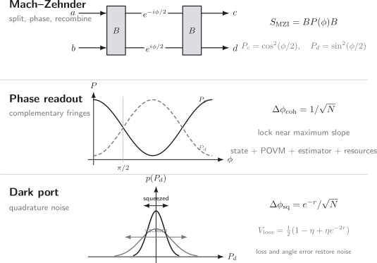
The Mach–Zehnder sequence maps a differential arm phase into complementary output probabilities. A coherent input supplies the inverse-square-root shot-noise baseline; a correctly oriented squeezed input reduces the dark-port quadrature noise. Loss and phase error mix ordinary vacuum or anti-squeezing back into the readout.

Single-Photon Interference

Output state

For one photon in input $a$ and vacuum in $b$, the Schrödinger output state in the chosen convention is

$$\begin{aligned} |\psi_{\mathrm{out}}(\phi)\rangle ={}& \cos\left(\frac\phi2\right) |1,0\rangle \\ &- i\sin\left(\frac\phi2\right) |0,1\rangle. \end{aligned}$$

Ideal output counting gives

$$\begin{aligned} p_c(\phi) &= \cos^2\left(\frac\phi2\right) = \frac{1+\cos\phi}{2}, \\ p_d(\phi) &= \sin^2\left(\frac\phi2\right) = \frac{1-\cos\phi}{2}. \end{aligned}$$

The probabilities sum to one. At $\phi=0$, output $c$ is bright and $d$ is dark; at $\phi=\pi$, their roles reverse. Each run produces one localized click, while repeated runs reconstruct the fringe.

Open and closed arrangements

After the first beam splitter, the photon occupies a coherent superposition of arm modes. Removing the second splitter measures in the arm basis and does not convert the relative phase into output populations. Inserting the second splitter measures in a phase-sensitive superposition basis.

This distinction is a change of measurement, not a retroactive change in what happened earlier. Delayed-choice interpretation is developed at Delayed-Choice Experiments.

Visibility

A common empirical model is

$$\begin{aligned} p_c(\phi) &= \frac12 \left[ 1+\mathcal V \cos(\phi+\phi_0) \right], \\ p_d(\phi) &= \frac12 \left[ 1-\mathcal V \cos(\phi+\phi_0) \right], \end{aligned}$$

where $0\leq\mathcal V\leq1$. The offset $\phi_0$ fixes the instrument’s reference phase. Reduced visibility can result from amplitude imbalance, mode mismatch, bandwidth averaging, unresolved path markers, or random phase noise. A fitted $\mathcal V$ alone does not identify which mechanism is responsible.

From Fringes to Phase Estimates

Local error propagation

Suppose an observable $\hat M$ has mean $m(\phi)$ and standard deviation $\Delta M$. Near a calibrated operating point $\phi_0$, the local error-propagation estimate is

$$\Delta\phi_{\mathrm{ep}} = \frac{ \Delta M }{ \left| \partial_\phi m \right| }_{\phi=\phi_0}.$$

This formula is a linearized property of a chosen observable. It is not a universal lower bound, and it can fail at a fringe extremum where the slope vanishes, for a biased estimator, or when the likelihood is multimodal.

An interferometer is commonly locked near a point with a large, stable slope. Feedback keeps the residual phase inside the locally invertible region, and calibration converts the error signal into physical phase.

Binary-count Fisher information

For one detected photon with the ideal probabilities above, the classical Fisher information is

$$\mathcal I_1(\phi) = \sum_{j=c,d} \frac{ \left[ \partial_\phi p_j(\phi) \right]^2 }{ p_j(\phi) }.$$

Away from the exact zero-probability endpoints, direct substitution gives

$$\mathcal I_1(\phi)=1.$$

The same value holds at the endpoints by a limiting argument. For $\nu$ independent detected photons,

$$\mathcal I_\nu=\nu,$$

and an unbiased locally efficient estimator satisfies

$$\Delta\phi \geq \frac1{\sqrt\nu}.$$

This calculation makes the resource explicit: $\nu$ is the number of independent detected one-photon trials. It does not include uncounted losses, state-preparation overhead, or a cost for finding the correct fringe.

Visibility reduces information

For the visibility model, the Fisher information per detected event is

$$\mathcal I_1(\phi) = \frac{ \mathcal V^2 \sin^2(\phi+\phi_0) }{ 1- \mathcal V^2 \cos^2(\phi+\phi_0) }.$$

At quadrature,

$$\phi+\phi_0 = \frac{\pi}{2},$$

so

$$\mathcal I_1=\mathcal V^2.$$

With $N_{\mathrm{det}}$ independent detected photons, the corresponding local bound is

$$\Delta\phi \geq \frac{ 1 }{ \mathcal V\sqrt{N_{\mathrm{det}}} }.$$

Unequal efficiencies and background counts require the full detector likelihood; they cannot always be represented by one visibility.

Quantum Fisher information

For a pure state that acquires phase through $e^{-i\phi\hat J_z}$, the quantum Fisher information is

$$F_Q = 4 \left( \Delta J_z \right)^2.$$

This is computed in the state inside the interferometer, after the first splitter and before the phase. It bounds the Fisher information of every possible output measurement:

$$\mathcal I(\phi)\leq F_Q.$$

For one photon split equally between the arms, $(\Delta J_z)^2=1/4$ and $F_Q=1$. Output photon counting therefore attains the available local information. General proofs and multiparameter cautions belong to Quantum Sensing.

Coherent Light and Shot Noise

Output state and mean counts

Send a coherent state $|\alpha\rangle$ into port $a$ and vacuum into port $b$. Let

$$\bar n=|\alpha|^2$$

be the mean input photon number in the selected measurement interval. Passive linear optics preserves the product-coherent form:

$$\begin{aligned} |\alpha,0\rangle \longmapsto{}& \left| \alpha\cos\left(\frac\phi2\right) \right\rangle_c \\ &\otimes \left| -i\alpha\sin\left(\frac\phi2\right) \right\rangle_d. \end{aligned}$$

The output means are

$$\begin{aligned} \overline n_c &= \bar n \cos^2\left(\frac\phi2\right), \\ \overline n_d &= \bar n \sin^2\left(\frac\phi2\right). \end{aligned}$$

Each output has Poisson statistics, and the two ideal coherent outputs are independent.

Difference readout

Define

$$\hat M = \hat n_c-\hat n_d.$$

Then

$$\langle\hat M\rangle = \bar n\cos\phi.$$

For independent Poisson outputs,

$$\begin{aligned} (\Delta M)^2 &= (\Delta n_c)^2 + (\Delta n_d)^2 \\ &= \overline n_c+\overline n_d = \bar n. \end{aligned}$$

The difference signal removes common mean intensity but not quantum fluctuations. At quadrature, $|\sin\phi|=1$, error propagation gives

$$\Delta\phi_{\mathrm{coh}} = \frac1{\sqrt{\bar n}}.$$

This is the coherent-state shot-noise scaling for one measurement interval. After many equal intervals, replace $\bar n$ by the total detected coherent photon number when the trials are independent and the phase is stable.

Full Poisson likelihood

The Fisher information in both output counts is

$$\mathcal I_{\mathrm{P}} = \sum_{j=c,d} \frac{ \left( \partial_\phi\overline n_j \right)^2 }{ \overline n_j }.$$

For the ideal coherent input,

$$\mathcal I_{\mathrm{P}}=\bar n.$$

The limiting value remains finite at a dark fringe even though difference signal error propagation has zero slope there. Near a dark port, the small mean count is quadratic in phase, and a full likelihood can estimate $|\phi|$. It cannot determine the sign without an offset, phase modulation, homodyne reference, or prior information.

What shot noise means

For an ideal coherent state, photon counts in a fixed mode and interval obey

$$\operatorname{Var}(N) = \langle N\rangle.$$

This Poisson variance is called optical shot noise. It remains when classical intensity noise, electronic noise, and environmental drift have been removed. “Shot-noise limited” means that the measured uncertainty agrees with a declared quantum-statistical model over a stated frequency and power range. It does not mean zero noise.

The phrase “standard quantum limit” is context dependent:

• for independent optical probes, it often means $1/\sqrt N$ phase scaling;
• for continuous displacement sensing, it can mean an optimum between measurement imprecision and radiation-pressure backaction;
• for clocks or spins, it often refers to projection noise of uncorrelated particles.

These baselines should not be conflated. The relevant detector, generator, bandwidth, and resource count must be named.

Standard Quantum Limit owns the general independent-probe derivation and resource audit; this page owns the optical counting model and interferometer-specific implementation.

Classical and technical noise

Real count or photocurrent variance can be written schematically as

$$V_{\mathrm{meas}} = V_{\mathrm{shot}} + V_{\mathrm{technical}} + V_{\mathrm{electronic}},$$

provided the contributions are independent and expressed in compatible units. Technical terms can include laser intensity noise, frequency noise converted by arm mismatch, vibration, thermal drift, beam pointing, scattered-light interference, and detector gain fluctuations.

Power scaling helps diagnose them. Coherent shot-noise amplitude grows as the square root of optical power, while many classical amplitude-noise terms grow linearly with power. That heuristic is not a substitute for calibrated noise injection and transfer-function measurements.

Phase Noise and Imperfect Contrast

Random phase

Let the actual phase be

$$\phi_{\mathrm{act}} = \phi+\delta\phi.$$

For zero-mean Gaussian phase noise with variance $\sigma_\phi^2$,

$$\left\langle e^{i\delta\phi} \right\rangle = e^{-\sigma_\phi^2/2}.$$

The averaged fringe is therefore

$$\langle\cos\phi_{\mathrm{act}}\rangle = e^{-\sigma_\phi^2/2} \cos\phi.$$

Fast phase noise reduces visibility. Slow drift can instead move the operating point between measurements and produce correlated, nonstationary errors. Treating every drift as independent Gaussian contrast loss can underestimate uncertainty.

Mode mismatch

Only overlapping output modes interfere. If one contribution decomposes into a component parallel to the other and an orthogonal remainder, the parallel component contributes to the fringe while the orthogonal part adds incoherent power. Spatial, temporal, spectral, and polarization overlap all matter.

A visibility loss is not automatically decoherence of the source. It may be ordinary mismatch in the measurement basis. Conversely, excellent average spatial overlap does not rule out hidden spectral or polarization markers.

Loss

Equal phase-independent loss after the interferometer reduces the detected photon number:

$$N_{\mathrm{det}} = \eta N_{\mathrm{in}}.$$

For a coherent input, the detected state remains coherent and the local phase uncertainty becomes

$$\Delta\phi_{\mathrm{loss}} = \frac1{\sqrt{\eta N_{\mathrm{in}}}}.$$

Unequal arm loss changes both visibility and the optimal operating point. Loss inside the arms can also carry path information into environmental modes. A trustworthy model places each loss channel at its physical location rather than attaching one efficiency to the final formula.

Squeezed-Input Improvement

Dark-port linearization

Take $\alpha$ real and bright in input $a$, and inject a zero-mean state into input $b$. Near the dark operating point $\phi=0$,

$$\begin{aligned} \hat d_{\mathrm{out}} &= -i\sin\left(\frac\phi2\right) \hat a \\ &\quad+ \cos\left(\frac\phi2\right) \hat b \\ &\approx \hat b-\frac{i\phi}{2}\hat a. \end{aligned}$$

Define

$$\hat P_d = \frac{ \hat d-\hat d^\dagger }{ i\sqrt2 }.$$

Replacing the bright carrier by its mean to leading order gives

$$\langle\hat P_d\rangle \approx -\frac{\alpha\phi}{\sqrt2}.$$

Vacuum in port $b$ has

$$\operatorname{Var}(P_b)=\frac12,$$

which recovers

$$\Delta\phi_{\mathrm{vac}} = \frac1{|\alpha|} = \frac1{\sqrt{\bar n}}.$$

If the measured quadrature of port $b$ is squeezed by $r$,

$$\operatorname{Var}(P_b) = \frac12e^{-2r},$$

then the ideal local uncertainty is

$$\Delta\phi_{\mathrm{sq}} = \frac{ e^{-r} }{ \sqrt{\bar n} }.$$

This is the Caves dark-port mechanism in its simplest linearized form. Direct photon counting exactly at a dark fringe has a quadratic response; homodyne readout, DC offset, RF modulation, or another phase reference provides a signed linear error signal.

Squeezing-angle error

If the squeezed ellipse is misaligned from the measured quadrature by $\epsilon$, the injected variance is

$$\begin{aligned} V(\epsilon) = \frac12 \left( e^{-2r}\cos^2\epsilon + e^{2r}\sin^2\epsilon \right). \end{aligned}$$

The anti-squeezed term grows rapidly with $r$. Increasing source squeezing without improving phase control can therefore worsen the measured noise.

Loss mixes in vacuum

For net efficiency $\eta$, a pure-loss channel gives

$$V_{\mathrm{det}} = \frac12 \left[ \eta e^{-2r} + 1-\eta \right].$$

If the same efficiency attenuates the signal slope, the local phase uncertainty becomes

$$\Delta\phi_{\mathrm{sq,loss}} = \frac{ \sqrt{ 1-\eta+\eta e^{-2r} } }{ \sqrt{\eta\bar n} }.$$

As $r\to\infty$, loss leaves a vacuum floor. Quoting source squeezing before propagation is therefore insufficient; the relevant quantity is the quadrature variance in the detected mode at the readout frequency.

Backaction and frequency dependence

In a static phase model, more carrier photons and stronger phase squeezing both improve imprecision. A movable mirror changes the problem. Carrier amplitude fluctuations exert radiation-pressure force, and squeezing the phase quadrature anti-squeezes the conjugate amplitude quadrature. At high power or low frequency, increased backaction can offset the imprecision gain.

Filter cavities and frequency-dependent readout can rotate the squeezing ellipse so that different quadratures are useful in different spectral regions. The full force-measurement tradeoff belongs to Optomechanics.

Other nonclassical inputs

Twin-Fock, Holland–Burnett, NOON, and other entangled number states can have larger phase-generator variance than independent photons. In an ideal fixed-$N$ model, suitably chosen states and measurements can approach $1/N$ local scaling.

That statement has strict qualifications:

• phase may be ambiguous over multiple fringes without prior information;
• preparation and detection resources must be counted;
• photon loss can destroy high-order coherence;
• the measurement that attains quantum Fisher information may be difficult;
• asymptotic scaling does not guarantee an advantage at finite $N$;
• indefinite-number resource constraints require special care.

This page does not assign one universal “Heisenberg limit.” The operational comparison is between complete protocols under the same declared resources and noise.

Readout Strategies

Two-port photon counting

Counting both outputs uses energy conservation and rejects some common-mode fluctuations. Number-resolving detectors provide the full joint count distribution; threshold detectors generally lose information at higher occupation. Detector efficiency, dark counts, dead time, saturation, and afterpulsing belong in the likelihood.

The dedicated Photon Counting page develops continuous records and jumps. The later optical photon-counting page will own laboratory counting POVMs and detector corrections.

Balanced homodyne

Homodyne detection mixes the signal output with a strong phase reference and measures a selected quadrature. It is natural for dark-port phase signals and squeezed inputs because it can choose the low-noise quadrature directly. Local-oscillator mode mismatch appears as loss, and phase error mixes in anti-squeezing.

Homodyne Detection owns the balanced difference current, stochastic record, and conditional state description.

Modulation and lock-in readout

A small known phase modulation can move the signal away from low-frequency technical noise and provide a signed error signal around a dark fringe. Demodulation estimates the response at the modulation frequency. The modulation depth, sideband transfer, detector bandwidth, and demodulation phase become part of the calibration.

Adaptive phase estimation

When the phase is not already localized to one fringe, a fixed operating point can be inefficient or ambiguous. Adaptive protocols update a controllable reference phase using previous outcomes. Bayesian or maximum likelihood estimators can then combine information across settings.

Adaptive performance depends on the prior, control latency, estimator, and loss. A local Cramér–Rao bound does not by itself certify globally reliable phase acquisition.

Applications to Metrology

Displacement

For one-way propagation in vacuum,

$$\phi = \frac{2\pi}{\lambda} \Delta L.$$

In a simple Michelson round trip, a mirror displacement $\Delta x$ changes the optical path by $2\Delta x$, giving

$$\phi = \frac{4\pi}{\lambda} \Delta x.$$

The inferred displacement uncertainty is

$$\Delta x = \frac{\lambda}{4\pi} \Delta\phi$$

for that ideal double-pass geometry. Cavities, folded paths, incidence angle, dispersion, and control loops modify the transfer function.

Refractive index and spectroscopy

A sample of length $L$ and refractive index $n(\omega)$ contributes

$$\phi(\omega) = \frac{\omega}{c} n(\omega)L.$$

Comparing it with a reference arm can reveal index changes, dispersion, absorption-induced contrast loss, or resonant phase shifts. Near a resonance, the full complex transfer function is required because amplitude and phase responses are linked and detector saturation or technical laser noise may dominate.

Rotation

Counterpropagating waves in a Sagnac loop enclose area $A$. For rotation component $\Omega$ normal to the loop, the ideal vacuum phase is

$$\phi_{\mathrm{Sag}} = \frac{ 8\pi A\Omega }{ \lambda c }.$$

Fiber coils increase effective area through multiple turns. Real gyroscopes must model polarization, backscatter, thermal gradients, scale-factor drift, and nonreciprocal phase shifts.

Gravitational-wave detectors

Kilometer-scale detectors use power-recycled Michelson interferometers with Fabry–Perot arm cavities, multiple control degrees of freedom, and frequency-dependent response. A gravitational wave produces a tiny differential arm-length signal. Quantum shot noise, radiation-pressure backaction, optical loss, mirror thermal noise, coating noise, seismic motion, and control noise contribute in different frequency bands.

Squeezed-vacuum injection is an operational quantum enhancement in current observatories, but its benefit is reported as part of a detector-wide strain noise spectrum and duty cycle, not as a free-standing squeezing parameter.

General transduction

If a physical parameter $\theta$ produces phase $\phi(\theta)$, then local uncertainties obey

$$\Delta\theta = \frac{ \Delta\phi }{ \left| \partial_\theta\phi \right| }.$$

Improvement can come from a steeper transduction coefficient, lower phase noise, more independent resources, or a better estimator. Calling every improvement “quantum enhanced” obscures which part of the measurement actually changed.

Bandwidth and Calibration

Dynamic response

A real interferometer has a frequency-dependent transfer function. In the Fourier domain, write

$$y(\Omega) = H_{\phi}(\Omega) \phi(\Omega) + n_y(\Omega),$$

where $y$ is the detector record, $H_\phi$ converts phase to output units, and $n_y$ is additive output noise. Calibration estimates $H_\phi$ and its uncertainty.

A static slope is sufficient only when the signal frequencies lie well inside the flat, linear response region. Cavity storage time, detector bandwidth, digital filters, feedback loops, and propagation delay can all alter magnitude and phase.

Spectral sensitivity

Amplitude spectral density is quoted per square root bandwidth, for example

$$\sqrt{S_\phi(\Omega)} \quad \text{in} \quad \mathrm{rad}/\sqrt{\mathrm{Hz}}.$$

An integrated root-mean-square uncertainty requires a bandwidth and filter:

$$\sigma_\phi^2 = \int_{\mathcal B} \frac{d\Omega}{2\pi} |F(\Omega)|^2 S_\phi(\Omega).$$

A single noise value without the one-sided or two-sided convention, bandwidth, integration time, and filtering cannot be compared reliably with another experiment.

Calibration chain

A defensible calibration records:

1. a traceable actuator or reference phase;
2. the optical response from actuator to detected signal;
3. detector gain, linearity, and saturation;
4. digital filtering and timing;
5. uncertainty and drift in every conversion;
6. injections that test the model over the signal band.

The final physical uncertainty combines statistical noise with calibration and systematic uncertainty. More photons reduce only the terms that truly average with photon number.

Practical Workflow

Before calculating

1. Declare the input, arm, output, and detector-selected modes.
2. State every beam-splitter and propagation phase convention.
3. Identify the physical parameter and derive $\phi(\theta)$.
4. Specify the input density operator and all inaccessible modes.
5. Place loss, phase noise, and mode mismatch at their physical locations.
6. Define the measured observable or POVM.
7. Write the complete outcome likelihood.
8. Choose a local or global estimator and its prior range.

Before claiming sensitivity

1. Report incident, intracavity, and detected resources separately.
2. Give contrast, efficiency, bandwidth, and integration time.
3. Show the noise spectrum or count model used for the uncertainty.
4. Distinguish raw data from loss-corrected or background-subtracted values.
5. Compare against a measured coherent or vacuum baseline under matched conditions.
6. Include estimator bias, dead time, calibration, and technical drift.
7. State whether the result improves variance, bandwidth, dynamic range, or a complete task-level figure of merit.

Common Mistakes

• Treating an isolated optical phase as observable without a reference.
• Adding arm probabilities instead of recombining amplitudes.
• Mixing beam-splitter phase conventions halfway through the Mach–Zehnder.
• Forgetting that the second splitter selects a phase-sensitive measurement basis.
• Calling a fringe extremum the most sensitive operating point because its contrast is visually large.
• Using error propagation where the signal slope vanishes and then claiming the interferometer contains no information.
• Quoting $1/\sqrt N$ without defining incident, circulating, or detected photon number and the integration interval.
• Calling all inverse-square-root scaling the same standard quantum limit.
• Subtracting common intensity noise and assuming quantum shot noise is also canceled.
• Inferring phase sensitivity from visibility alone.
• Treating slow drift as independent noise that averages down indefinitely.
• Calling all loss a final detector inefficiency even when arm loss reveals path information.
• Quoting generated squeezing instead of detected mode-matched squeezing.
• Ignoring anti-squeezing leaked by phase jitter.
• Claiming $1/N$ scaling without a global phase strategy, fair resources, or a loss model.
• Converting a phase spectrum to an rms uncertainty without bandwidth and spectral-density conventions.
• Reporting a statistical fit error while omitting calibration and systematic uncertainty.

Connections

• Mach–Zehnder Interferometry audits optical phase sensing as an end-to-end estimation protocol, including references, global ambiguity, loss bounds, multipass queries, and sample disturbance.
• Beam Splitters owns the two-port unitary, phase conventions, and Fock-state transformations used by each mixer.
• Coherent Light owns coherent amplitudes, Poisson statistics, phase references, and passive-network propagation.
• Squeezed Light develops quadrature squeezing, dark-port injection, loss, and experimental verification.
• Phase-Space Distributions provides the Gaussian and quasidistribution view of passive mode transformations and homodyne readout.
• Fisher Information develops scores, additivity, Cramér–Rao bounds, and regularity assumptions.
• Quantum Sensing owns general quantum Fisher information, decoherence limits, and sensing resource comparisons.
• Interferometry surveys optical and matter-wave instrument families and their historical role.
• Ramsey Interferometry develops the two-pulse internal-state interferometer and clock error signal.
• Entanglement in Quantum Optics owns path-mode entanglement and nonclassical optical resources.
• Homodyne Detection develops quadrature records and detector efficiency.
• Optomechanics develops displacement imprecision, radiation-pressure backaction, and the continuous-measurement standard quantum limit.

Exercises

1. Multiply the Mach–Zehnder matrices

Using

$$B = \frac1{\sqrt2} \begin{pmatrix} 1&1\\ 1&-1 \end{pmatrix}$$

and

$$P(\phi) = \begin{pmatrix} e^{-i\phi/2}&0\\ 0&e^{i\phi/2} \end{pmatrix},$$

derive $S_{\mathrm{MZI}}=BPB$. Check $\phi=0$ and $\phi=\pi$.

Solution

First multiply on the right:

$$P B = \frac1{\sqrt2} \begin{pmatrix} e^{-i\phi/2}&e^{-i\phi/2}\\ e^{i\phi/2}&-e^{i\phi/2} \end{pmatrix}.$$

Let

$$z=e^{-i\phi/2}.$$

Then

$$\begin{aligned} B P B &= \frac12 \begin{pmatrix} z+z^* & z-z^* \\ z-z^* & z+z^* \end{pmatrix} \\ &= \begin{pmatrix} \cos(\phi/2)&-i\sin(\phi/2)\\ -i\sin(\phi/2)&\cos(\phi/2) \end{pmatrix}. \end{aligned}$$

At $\phi=0$, this is the identity. At $\phi=\pi$,

$$S_{\mathrm{MZI}}(\pi) = \begin{pmatrix} 0&-i\\ -i&0 \end{pmatrix},$$

which swaps the ports and attaches a convention-dependent phase $-i$.

2. Single-photon Fisher information

For

$$p_c = \cos^2\left(\frac\phi2\right), \qquad p_d = \sin^2\left(\frac\phi2\right),$$

calculate the Fisher information per detected photon. Why should the exact dark-fringe points be handled by a limit?

Solution

The derivatives are

$$\partial_\phi p_c = -\frac12\sin\phi, \qquad \partial_\phi p_d = \frac12\sin\phi.$$

Therefore

$$\begin{aligned} \mathcal I_1 ={}& \frac{ \sin^2\phi }{ 4\cos^2(\phi/2) } \\ &+ \frac{ \sin^2\phi }{ 4\sin^2(\phi/2) }. \end{aligned}$$

Using

$$\sin^2\phi = 4 \sin^2\left(\frac\phi2\right) \cos^2\left(\frac\phi2\right)$$

gives

$$\mathcal I_1 = \sin^2\left(\frac\phi2\right) + \cos^2\left(\frac\phi2\right) =1.$$

At $\phi=0$ or $\pi$, one displayed denominator and its numerator both vanish. The original likelihood is well defined, but the algebraic Fisher formula must be interpreted by the neighboring-phase limit. Globally, those points also retain a sign ambiguity unless an offset or prior is supplied.

3. Coherent difference-count sensitivity

A coherent state with mean input number $\bar n$ enters port $a$. Derive the mean and variance of $\hat M=\hat n_c-\hat n_d$. Find the error-propagation phase uncertainty and identify its best operating point.

Solution

The output means are

$$\begin{aligned} \overline n_c &= \bar n\cos^2\left(\frac\phi2\right), \\ \overline n_d &= \bar n\sin^2\left(\frac\phi2\right). \end{aligned}$$

Hence

$$\langle M\rangle = \overline n_c-\overline n_d = \bar n\cos\phi.$$

The two coherent outputs have independent Poisson counts, so

$$\begin{aligned} (\Delta M)^2 &= (\Delta n_c)^2 + (\Delta n_d)^2 \\ &= \overline n_c+\overline n_d = \bar n. \end{aligned}$$

Because

$$\left| \partial_\phi\langle M\rangle \right| = \bar n|\sin\phi|,$$

error propagation gives

$$\Delta\phi_{\mathrm{ep}} = \frac{ 1 }{ \sqrt{\bar n}|\sin\phi| }.$$

It is minimized at quadrature, $\phi=\pi/2$ or $3\pi/2$, where

$$\Delta\phi_{\mathrm{ep}} = \frac1{\sqrt{\bar n}}.$$

The divergence at a fringe extremum is a failure of this signed difference observable’s linear slope, not proof that the full count distribution has zero local Fisher information.

4. Contrast and detected resources

For

$$p_\pm = \frac12 \left[ 1\pm\mathcal V\cos\phi \right],$$

derive the Fisher information per detected photon. Evaluate it at quadrature and include a phase-independent detection efficiency $\eta$ for $N_{\mathrm{in}}$ incident independent photons.

Solution

The derivatives are

$$\partial_\phi p_\pm = \mp\frac{\mathcal V}{2}\sin\phi.$$

Since

$$p_+p_- = \frac14 \left( 1-\mathcal V^2\cos^2\phi \right),$$

the binary Fisher information is

$$\mathcal I_1(\phi) = \frac{ \mathcal V^2\sin^2\phi }{ 1-\mathcal V^2\cos^2\phi }.$$

At quadrature,

$$\mathcal I_1=\mathcal V^2.$$

If loss only removes events independently, the expected detected resource is

$$N_{\mathrm{det}} = \eta N_{\mathrm{in}}.$$

The local Cramér–Rao bound becomes

$$\Delta\phi \geq \frac{ 1 }{ \mathcal V \sqrt{\eta N_{\mathrm{in}}} }.$$

This simple factorization fails when loss is arm dependent, phase dependent, or correlated with another degree of freedom.

5. Gaussian phase jitter

Let $\delta\phi$ be a zero-mean Gaussian random variable of variance $\sigma_\phi^2$. Show how averaging over it changes an ideal $\cos\phi$ fringe. What is the small-noise visibility loss?

Solution

The Gaussian characteristic function is

$$\left\langle e^{i\delta\phi} \right\rangle = e^{-\sigma_\phi^2/2}.$$

Therefore

$$\begin{aligned} \left\langle \cos(\phi+\delta\phi) \right\rangle &= \operatorname{Re} \left[ e^{i\phi} \left\langle e^{i\delta\phi} \right\rangle \right] \\ &= e^{-\sigma_\phi^2/2} \cos\phi. \end{aligned}$$

The effective visibility is

$$\mathcal V_{\mathrm{eff}} = e^{-\sigma_\phi^2/2}.$$

For $\sigma_\phi\ll1$,

$$\mathcal V_{\mathrm{eff}} \approx 1-\frac{\sigma_\phi^2}{2}.$$

This averaging model describes phase jitter fast enough to be sampled by the data ensemble. Slow drift creates correlated errors and should be modeled as a time-dependent nuisance parameter instead.

6. Squeezing angle and loss

A dark-port input has squeezed and anti-squeezed variances $e^{-2r}/2$ and $e^{2r}/2$. Derive the measured quadrature variance for angle error $\epsilon$, then include pure-loss efficiency $\eta$. Explain why large $r$ demands tighter phase control.

Solution

Resolving the measured quadrature along the principal axes gives

$$V(\epsilon) = \frac12 \left( e^{-2r}\cos^2\epsilon + e^{2r}\sin^2\epsilon \right).$$

Pure loss mixes the state with vacuum variance $1/2$:

$$\begin{aligned} V_\eta(\epsilon) &= \eta V(\epsilon) + \frac{1-\eta}{2} \\ &= \frac12 \bigl[ \eta e^{-2r}\cos^2\epsilon \\ &\quad+ \eta e^{2r}\sin^2\epsilon + 1-\eta \bigr]. \end{aligned}$$

For small angle error,

$$\sin^2\epsilon\approx\epsilon^2.$$

The leaked anti-squeezed contribution is then approximately $\eta e^{2r}\epsilon^2/2$. It grows exponentially with $r$, so a source with stronger nominal squeezing can perform worse unless phase noise is reduced at the same time. Loss also creates a floor that cannot be removed by increasing $r$.

7. Generator variance for independent photons

After the first balanced splitter, one photon occupies

$$|\psi\rangle = \frac{ |1,0\rangle+|0,1\rangle }{ \sqrt2 }$$

inside the arms. Compute $(\Delta J_z)^2$ for $\hat J_z=(\hat n_u-\hat n_\ell)/2$. Extend the result to $N$ independent photons and obtain the quantum Fisher information.

Solution

For one photon, the two possible $J_z$ eigenvalues are $+1/2$ and $-1/2$, each with probability $1/2$. Thus

$$\langle J_z\rangle=0$$

and

$$\left( \Delta J_z \right)^2 = \frac12 \left( \frac14+\frac14 \right) = \frac14.$$

The pure-state quantum Fisher information is

$$F_Q = 4 \left( \Delta J_z \right)^2 =1.$$

For $N$ independent photons, variances add:

$$\left( \Delta J_z^{(N)} \right)^2 = \frac N4.$$

Therefore

$$F_Q^{(N)}=N, \qquad \Delta\phi\geq\frac1{\sqrt N}.$$

Correlations can change the total generator variance, but whether that variance yields an operational advantage depends on preparation, measurement, loss, and global phase ambiguity.

8. Displacement sensitivity and noise budget

A simple Michelson interferometer uses wavelength $\lambda=1064\,\mathrm{nm}$ and detects $N_{\mathrm{det}}=10^{12}$ coherent photons in one integration interval. Ignoring all other noise, estimate the shot-noise-limited mirror displacement uncertainty. Then state three reasons this is not yet a detector sensitivity claim.

Solution

The coherent phase uncertainty is

$$\Delta\phi = \frac1{\sqrt{N_{\mathrm{det}}}} = 10^{-6}\,\mathrm{rad}.$$

For a double-pass Michelson,

$$\phi = \frac{4\pi}{\lambda}x,$$

so

$$\begin{aligned} \Delta x &= \frac{\lambda}{4\pi} \Delta\phi \\ &= \frac{ 1064\times10^{-9}\,\mathrm m }{ 4\pi } 10^{-6} \\ &\approx 8.5\times10^{-14}\,\mathrm m. \end{aligned}$$

This is not yet a complete sensitivity claim because, among other issues:

• the integration time and equivalent bandwidth were not specified;
• contrast, optical loss, detector efficiency, and calibration uncertainty were assumed ideal;
• vibration, laser frequency and intensity noise, thermal noise, scattered light, and radiation-pressure backaction were omitted.

It is a useful quantum-statistical baseline for the stated detected photon resource, not a prediction for a full instrument.

References

1. B. Yurke, S. L. McCall, and J. R. Klauder, “SU(2) and SU(1,1) Interferometers,” Physical Review A 33, 4033–4054 (1986), doi:10.1103/PhysRevA.33.4033.
2. C. M. Caves, “Quantum-Mechanical Noise in an Interferometer,” Physical Review D 23, 1693–1708 (1981), doi:10.1103/PhysRevD.23.1693.
3. M. J. Holland and K. Burnett, “Interferometric Detection of Optical Phase Shifts at the Heisenberg Limit,” Physical Review Letters 71, 1355–1358 (1993), doi:10.1103/PhysRevLett.71.1355.
4. S. L. Braunstein and C. M. Caves, “Statistical Distance and the Geometry of Quantum States,” Physical Review Letters 72, 3439–3443 (1994), doi:10.1103/PhysRevLett.72.3439.
5. V. Giovannetti, S. Lloyd, and L. Maccone, “Advances in Quantum Metrology,” Nature Photonics 5, 222–229 (2011), doi:10.1038/nphoton.2011.35.
6. L. Pezzè, A. Smerzi, M. K. Oberthaler, R. Schmied, and P. Treutlein, “Quantum Metrology with Nonclassical States of Atomic Ensembles,” Reviews of Modern Physics 90, 035005 (2018), doi:10.1103/RevModPhys.90.035005.
7. R. Schnabel, “Squeezed States of Light and Their Applications in Laser Interferometers,” Physics Reports 684, 1–51 (2017), doi:10.1016/j.physrep.2017.04.001.
8. M. Tse et al., “Quantum-Enhanced Advanced LIGO Detectors in the Era of Gravitational-Wave Astronomy,” Physical Review Letters 123, 231107 (2019), doi:10.1103/PhysRevLett.123.231107.
9. L. Mandel and E. Wolf, Optical Coherence and Quantum Optics (Cambridge University Press, 1995), Chapters 9, 12, and 22, doi:10.1017/CBO9781139644105.
10. C. C. Gerry and P. L. Knight, Introductory Quantum Optics (Cambridge University Press, 2005), Chapters 6 and 11, doi:10.1017/CBO9780511791239.
11. D. F. Walls and G. J. Milburn, Quantum Optics, 2nd ed. (Springer, 2008), Chapters 2 and 6, doi:10.1007/978-3-540-28574-8.
12. C. W. Helstrom, Quantum Detection and Estimation Theory (Academic Press, 1976), Chapters 7 and 8.
13. H. M. Wiseman and G. J. Milburn, Quantum Measurement and Control (Cambridge University Press, 2010), Chapters 4 and 9, doi:10.1017/CBO9780511813948.