Homodyne and Heterodyne Detection

Homodyne detection measures one phase-selected field quadrature by interfering a signal with a strong coherent reference and subtracting two photodetector outputs. Heterodyne detection shifts the reference frequency and extracts two electronic quadratures, or equivalently divides the signal and performs two orthogonal homodyne measurements. The second method returns a complex amplitude in every trial, but the simultaneous readout necessarily contains one additional vacuum mode.

These are not merely bright-field versions of photon counting. Direct photodetection is naturally sensitive to normally ordered intensity and arrival events. A phase-sensitive receiver uses the local oscillator to convert a field amplitude into a macroscopic photocurrent. It can therefore measure vacuum fluctuations, squeezing, coherent displacements, and complete quadrature distributions even when the signal itself carries much less than one photon per selected mode on average.

A trustworthy quadrature measurement must state more than the receiver name. It must identify

• the spatial, temporal, spectral, and polarization mode selected by the local oscillator;
• the quadrature normalization and local-oscillator phase convention;
• how vacuum or shot noise was calibrated;
• the optical efficiency, visibility, detector balance, and electronic-noise model;
• whether the local-oscillator phase was fixed, scanned, or inferred;
• whether reported data are raw detector outcomes, loss-corrected estimates, or a reconstructed state.

The essential distinction is concise:

$$\begin{gathered} \text{homodyne: }x_\theta \\ \text{one quadrature per trial}, \\[4pt] \text{heterodyne: }(x_{\rm h},p_{\rm h}) \\ \text{one added vacuum contribution}. \end{gathered}$$

Canonical Scope

This page is the canonical home for practical optical quadrature receivers:

• the local oscillator as phase reference, gain field, and mode selector;
• the balanced-homodyne difference-current derivation;
• ideal quadrature outcome distributions and representative state examples;
• vacuum calibration, common-mode rejection, detector linearity, optical loss, imperfect overlap, phase noise, and electronic noise;
• pulsed-mode and continuous-wave implementations;
• detuned and dual-homodyne realizations of heterodyne detection;
• the coherent-state POVM, Husimi distribution, and heterodyne added vacuum;
• the operational connection between quadrature data and state tomography.

Beam Splitters owns the lossless two-port unitary and phase-convention bookkeeping. Phase-Space Distributions owns the full Glauber–Sudarshan, Wigner, and Husimi formalism, including tomographic inversion. Squeezed Light owns optical squeezing generation and its source-specific diagnostics.

The pages on Homodyne Detection and Heterodyne Detection in the open-systems volume instead own continuous stochastic records, conditional states, and diffusive quantum trajectories. The present page stops at the receiver outcome and the statistical state inference built from many such outcomes.

Quadrature Convention

Let $\hat a$ denote the annihilation operator of one declared optical mode, with

$$[\hat a,\hat a^\dagger]=1.$$

Use dimensionless canonical quadratures

$$\hat X = \frac{\hat a+\hat a^\dagger}{\sqrt2}, \qquad \hat P = \frac{\hat a-\hat a^\dagger}{i\sqrt2},$$

so that

$$[\hat X,\hat P]=i.$$

The quadrature at phase $\theta$ is

$$\begin{aligned} \hat X_\theta &= \frac{ \hat a e^{-i\theta} + \hat a^\dagger e^{i\theta} }{ \sqrt2 } \\ &= \hat X\cos\theta+\hat P\sin\theta. \end{aligned}$$

Its conjugate is $\hat X_{\theta+\pi/2}$. For the vacuum and every coherent state,

$$\operatorname{Var}(\hat X_\theta)=\frac12.$$

Some literature instead defines $\hat X=\hat a+\hat a^\dagger$, giving vacuum variance $1$. Others divide once more and quote vacuum variance $1/4$. Decibel squeezing values are unchanged when signal and vacuum use the same normalization, but raw variances and stochastic-record coefficients are not. The convention must therefore travel with every formula and data set.

The Local Oscillator

A local oscillator, abbreviated LO, is a coherent field prepared in the mode to which the receiver should be sensitive. Write its complex amplitude as

$$\beta = |\beta|e^{i\theta}.$$

The magnitude $|\beta|$ supplies measurement gain and the phase $\theta$ selects the quadrature. Three roles should be kept distinct.

A relational phase reference

The phase of an isolated optical mode is not measured against an absolute clock at hundreds of terahertz. It is measured relative to another field. A stable LO realizes that reference. Changing its phase rotates the measured axis in optical phase space; losing the shared reference averages phase-sensitive features over $\theta$.

For a coherent signal $|\alpha\rangle$, the homodyne mean is

$$\langle \hat X_\theta\rangle = \sqrt2\, \operatorname{Re}\!\left( \alpha e^{-i\theta} \right).$$

Thus a phase scan traces the projection of the coherent displacement onto a rotating axis. It does not reveal an observer-independent global optical phase.

A mode selector

Interference occurs only between mutually coherent field components. The LO therefore defines which combination of spatial profile, polarization, spectrum, and temporal envelope contributes coherently to the difference current. Orthogonal components add direct-detection noise or loss but not the desired phase-sensitive signal.

For a continuous output field satisfying

$$[ \hat a_{\rm out}(t), \hat a_{\rm out}^\dagger(t') ] = \delta(t-t'),$$

a normalized temporal mode $g(t)$ defines

$$\hat a_g = \int dt\, g^*(t)\hat a_{\rm out}(t).$$

Normalization gives

$$\int dt\,|g(t)|^2=1.$$

The effective $g(t)$ depends on the LO envelope, optical propagation, detector response, and electronic weighting used to integrate the current. A pulsed experiment that reports “the quadrature of the pulse” is therefore really reporting the quadrature of this selected mode.

If the intended signal mode is $u_s$ and the normalized LO mode is $u_{\rm LO}$, their complex overlap is

$$\mu = \langle u_{\rm LO},u_s\rangle.$$

After adjusting the phase, $|\mu|^2$ acts as a mode-matching efficiency. A high photodiode quantum efficiency cannot repair poor mode overlap.

A linear measurement gain

Photodiodes measure intensity. Interference with a bright LO produces a term linear in the weak signal field and proportional to $|\beta|$. Increasing LO power can raise this optical signal above electronic noise, but only while the photodiodes, transimpedance amplifiers, subtraction stage, and digitizer remain linear.

A stronger LO does not reduce the signal mode’s quantum uncertainty. It amplifies the quadrature and its quantum fluctuations together. Once electronic noise is negligible, further LO power gives no ideal improvement in quadrature signal-to-noise ratio and may instead cause saturation, heating, or imperfectly rejected classical intensity noise.

Balanced Homodyne Detection

The standard receiver combines the signal and LO on a balanced beam splitter, detects both outputs, and subtracts the resulting photocharges or photocurrents.

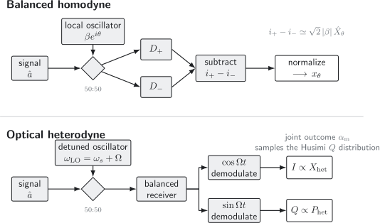
Balanced homodyne detection subtracts two outputs to isolate the quadrature $X_\theta$ selected by the local oscillator. A detuned heterodyne receiver demodulates the beat note in two electronic phases, producing a joint complex outcome with an unavoidable vacuum contribution.

Exact difference operator

Let $\hat a$ be the signal input and $\hat b$ the LO input. Choose the balanced-beam-splitter convention

$$\hat c = \frac{\hat a+\hat b}{\sqrt2}, \qquad \hat d = \frac{\hat b-\hat a}{\sqrt2}.$$

The output number difference is exactly

$$\begin{aligned} \hat n_c-\hat n_d &= \hat c^\dagger\hat c-\hat d^\dagger\hat d \\ &= \hat a^\dagger\hat b + \hat b^\dagger\hat a. \end{aligned}$$

The individual outputs contain the large LO intensity, whereas that common term cancels in the difference. For an LO coherent state with $\hat b\rightarrow\beta=|\beta|e^{i\theta}$,

$$\hat n_c-\hat n_d \longrightarrow \sqrt2\,|\beta|\,\hat X_\theta.$$

The normalized number difference therefore approaches

$$\hat X_\theta = \lim_{|\beta|\to\infty} \frac{ \hat n_c-\hat n_d }{ \sqrt2\,|\beta| }.$$

Different beam-splitter phase conventions may replace $\theta$ by $\theta+\pi/2$ or reverse the current sign. Those changes do not alter the measurement; they change the calibrated phase origin.

Why subtraction matters

Subtraction has two simultaneous functions:

1. It removes the mean LO intensity, leaving the signal–LO interference term.
2. It rejects fluctuations common to both photodiode channels.

The second statement is conditional. If the optical splitting ratio, detector responsivities, electronic gains, or time delays differ, LO intensity noise leaks into the difference channel. The residual is often negligible near the shot-noise band and severe at low Fourier frequency. “Balanced” is therefore an experimentally verified operating condition, not merely the presence of two detectors.

The sum channel is also useful:

$$\hat n_c+\hat n_d = \hat a^\dagger\hat a+\hat b^\dagger\hat b.$$

For a weak signal it monitors LO power and can reveal clipping, power drift, or photodiode mismatch. Normalizing every sample by a noisy instantaneous sum, however, changes the estimator and must be justified rather than applied automatically.

The strong-LO approximation

Write the LO operator as a displacement plus fluctuations,

$$\hat b=\beta+\delta\hat b.$$

Then

$$\begin{aligned} \hat n_c-\hat n_d ={}& \sqrt2\,|\beta|\,\hat X_\theta \\ &+ \hat a^\dagger\delta\hat b + \delta\hat b^\dagger\hat a. \end{aligned}$$

The first term scales as $|\beta|$; the remaining operator is finite as the LO is increased. In the strong-LO limit, the rescaled output statistics converge to the signal quadrature distribution. At finite LO power, the exact two-mode photodetection model should be retained when the signal is not weak relative to the LO or when high-order moments are required.

Treating $\hat b$ as a number does not mean the LO is noiseless. The limiting quadrature distribution already contains the appropriate quantum fluctuations, and photodetection of the bright coherent reference produces shot noise. The approximation means that LO depletion and finite-reference corrections are negligible.

Measuring Quadratures

An ideal homodyne measurement at phase $\theta$ has the projection-valued measure

$$E_\theta(dx) = |x;\theta\rangle \langle x;\theta|\,dx,$$

where

$$\hat X_\theta|x;\theta\rangle = x|x;\theta\rangle.$$

For a signal state $\rho$, the outcome density is

$$p_\theta(x) = \langle x;\theta|\rho|x;\theta\rangle.$$

It is normalized:

$$\int_{-\infty}^{\infty}dx\,p_\theta(x)=1.$$

The detector returns samples from $p_\theta(x)$, not merely its mean and variance. Histograms can expose non-Gaussian structure that a noise-power measurement misses.

Vacuum

In the present convention,

$$p_{\rm vac}(x) = \frac{1}{\sqrt\pi}e^{-x^2},$$

with

$$\langle x\rangle=0, \qquad \operatorname{Var}(x)=\frac12.$$

Vacuum is therefore not represented by a delta function at zero. Its finite width is the shot-noise reference against which optical squeezing is quoted.

Coherent state

For $|\alpha\rangle$, define its projected mean

$$\bar x_\theta = \sqrt2\, \operatorname{Re}(\alpha e^{-i\theta}).$$

The outcome density is

$$p_\theta(x|\alpha) = \frac{1}{\sqrt\pi} \exp\!\left[ - (x-\bar x_\theta)^2 \right].$$

The phase-dependent mean moves, while the variance remains $1/2$. A coherent state is therefore displaced vacuum in homodyne statistics.

Photon-number state

For a number state $|n\rangle$,

$$p_n(x) = \frac{ e^{-x^2} }{ \sqrt\pi\,2^n n! } H_n^2(x),$$

where $H_n$ is a Hermite polynomial. The distribution is independent of $\theta$ because a number state is invariant under phase rotation up to a global phase. For $n=1$ it vanishes at $x=0$ and has two lobes, a feature that cannot be inferred from variance alone.

Squeezed Gaussian state

Let $\phi$ denote the principal squeezed-axis angle, and let $r\geq0$ be the squeeze parameter. A pure squeezed vacuum has

$$\begin{aligned} \operatorname{Var}(\hat X_\theta) ={}& \frac12 e^{-2r} \cos^2(\theta-\phi) \\ &+ \frac12 e^{2r} \sin^2(\theta-\phi). \end{aligned}$$

At $\theta=\phi$, the variance is $e^{-2r}/2$; at the orthogonal phase it is $e^{2r}/2$. The uncertainty area is preserved even though one marginal is narrower than vacuum. Squeezed Light develops the generation and interpretation of these states.

Moments from samples

At fixed phase, ideal samples estimate symmetrically ordered quadrature moments:

$$\frac1N\sum_{j=1}^{N}x_j^k \longrightarrow \operatorname{Tr} \left( \rho\,\hat X_\theta^k \right).$$

Finite-sample uncertainty grows rapidly with $k$, especially for states with long tails. High-order moment estimates are also sensitive to digitizer clipping and incorrect electronic-baseline subtraction. Preserving the raw time series and detector metadata is usually more valuable than retaining only a processed variance.

Calibration and Nonidealities

An ideal quadrature POVM is a limiting description of an optical receiver. Real voltage samples must first be mapped to dimensionless $x_\theta$. That map should be established with independent calibration data, not adjusted until a desired state appears.

Vacuum and shot-noise calibration

Replace the signal by vacuum while leaving the LO path, detector settings, filtering, and digitizer range unchanged. If a measured voltage sample is

$$V=G X_\theta+V_{\rm el},$$

then the optical gain $G$ converts dimensionless quadrature into volts and $V_{\rm el}$ represents additive electronic noise. With independent, zero-mean terms,

$$\operatorname{Var}(V_{\rm vac}) = \frac{G^2}{2} + \operatorname{Var}(V_{\rm el}).$$

Because $G\propto|\beta|$, the optical vacuum contribution is proportional to LO power $P_{\rm LO}$. A useful receiver characterization measures the difference-noise variance over a range of LO powers and tests

$$\operatorname{Var}(V_{\rm diff}) = A P_{\rm LO} + B P_{\rm LO}^2 + V_{\rm el}.$$

The linear term is the expected shot-noise scaling. The constant intercept is electronic noise. A significant quadratic term often indicates leaked LO relative-intensity noise, although other nonlinearities can mimic it. At high power, compression can bend the curve downward. The operating interval should be chosen where the detector is linear, shot noise dominates the electronics, and classical excess noise remains rejected.

Blocking the LO as well as the signal measures electronics; it does not measure optical vacuum noise. Blocking or extinguishing the signal while retaining the LO leaves the signal input in vacuum and supplies the proper optical reference.

There are two common reporting conventions:

• normalize raw variances to the raw vacuum trace, leaving electronic noise in both numerator and denominator;
• estimate the electronic contribution with the LO off, subtract it from both variances, and normalize to the inferred optical shot noise.

The first is conservative but can hide modest squeezing by pulling ratios toward one. The second can overstate squeezing when two large, uncertain numbers are subtracted. A mature analysis reports the convention, clearance, uncertainty, and raw calibration data. Modeling electronics in the detector likelihood is preferable when tomography is the goal.

Loss and mode mismatch

Linear optical loss with total efficiency $\eta$ is equivalent to mixing the selected signal mode with vacuum:

$$\hat X_{\rm meas} = \sqrt\eta\,\hat X_{\rm sig} + \sqrt{1-\eta}\,\hat X_{\rm vac}.$$

Consequently,

$$\begin{aligned} \langle \hat X_{\rm meas}\rangle &= \sqrt\eta\, \langle \hat X_{\rm sig}\rangle, \\ V_{\rm meas} &= \eta V_{\rm sig} + \frac{1-\eta}{2}. \end{aligned}$$

The total efficiency can include propagation, optical transmission, photodiode quantum efficiency, and mode overlap:

$$\eta_{\rm tot} \simeq \eta_{\rm prop}\, \eta_{\rm opt}\, \eta_{\rm det}\, |\mu|^2.$$

This factorization is an experimental model, not an identity. Spatially or temporally varying detector response, excess noise in unmatched modes, and frequency-dependent loss can require a multimode treatment.

Loss drives every quadrature variance toward $1/2$ and smooths non-Gaussian features. Algebraically inverting the variance formula is possible when $\eta$ is known, but full loss inversion amplifies statistical and calibration errors and can yield an unphysical reconstructed density operator. It is often clearer to report the state at the detector input and separately infer the source state with an explicit uncertainty model.

Phase uncertainty

Suppose the intended LO phase is the squeezed-axis angle $\phi$, but the actual phase has a zero-mean Gaussian error $\delta\theta$ of variance $\sigma_\theta^2$. If the principal quadrature variances are $V_s$ and $V_a$, the averaged measured variance before loss is

$$\overline V = \frac{V_s+V_a}{2} + \frac{V_s-V_a}{2} e^{-2\sigma_\theta^2}.$$

Even small phase noise can matter when $V_a\gg V_s$: anti-squeezed noise leaks into the nominally squeezed record. A single “phase-lock bandwidth” does not fully specify this effect. The relevant phase-error spectrum must be weighted by the measurement interval and temporal mode.

Slow phase drift broadens a long-run histogram and can imitate a mixed state. Postselecting or rotating samples using an auxiliary phase estimate may be valid, but then that estimator and its uncertainty are part of the measurement model.

Balance, common-mode rejection, and linearity

A practical balanced receiver needs matched optical powers, photodiode responsivities, electronic gains, delays, and bandwidths. Its common-mode-rejection ratio should be measured at the Fourier frequencies used in the analysis. A large low-frequency specification does not guarantee good rejection across the full detection band.

Important checks include:

• vary LO power and verify linear mean response and linear shot-noise variance;
• inject a known LO amplitude modulation and measure its leakage into the difference channel;
• inspect each photodiode and the difference output for clipping;
• reverse the signal displacement or LO phase and verify the expected sign change;
• record dark electronics, vacuum, and a known coherent displacement with the same filters and digitizer settings;
• confirm that the inferred vacuum variance is stationary across the data run.

Detector saturation can narrow histograms and falsely suggest squeezing. Rare clipping can strongly bias fourth and higher moments while barely changing the variance. A histogram that ends abruptly at the digitizer rails is a hardware warning, not a non-Gaussian quantum feature.

Electronic filtering

The receiver does not measure an infinitely broad operator. Let the difference current be $i_-(t)$ and let $w(t)$ be the normalized electronic weight assigned to one trial. A pulsed outcome has the form

$$x_k = \mathcal N \int_{T_k}dt\, w(t)i_-(t),$$

where $\mathcal N$ is fixed by vacuum calibration. The optical LO envelope and $w(t)$ jointly define the temporal mode. Orthogonal temporal modes are discarded only if the receiver and integration really reject them.

Electronic high-pass filtering can introduce negative temporal lobes and correlations between adjacent pulse samples. Low-pass filtering can mix neighboring pulses. The same filter must be included when estimating independent sample count, uncertainty, and a tomographic likelihood.

Pulsed and Continuous-Wave Modes

The phrase “homodyne quadrature” covers two experimentally distinct measurement geometries.

Pulsed homodyne detection

In time-domain pulsed homodyne detection, each LO pulse gates one selected wave-packet mode. The integrated difference charge gives approximately one quadrature sample per pulse. Good mode matching requires overlap in

• transverse spatial profile and wavefront;
• polarization;
• carrier frequency and spectral phase;
• arrival time and temporal envelope.

Pulse-energy fluctuations are common-mode noise only to the degree that the receiver is balanced. If the signal mode is inferred from data, for example by principal-component analysis of time traces, the training and validation sets should be separated to avoid fitting detector noise.

Continuous-wave spectral homodyne detection

For a continuous-wave LO, one often analyzes the difference current at radio frequency $\Omega$. In a frame rotating at the LO frequency, the positive frequency component has the structure

$$\hat i_-(\Omega) \propto \beta^*\hat a(+\Omega) + \beta\,\hat a^\dagger(-\Omega).$$

The analysis therefore couples the upper and lower optical sidebands at $\omega_{\rm LO}\pm\Omega$. The measured cosine and sine electronic components are quadratures of sideband supermodes selected by the filter and demodulation phase. They should not automatically be interpreted as the quadratures of one infinitely sharp optical-frequency mode.

Spectral squeezing is reported by comparing the current-noise spectral density with the vacuum spectrum under identical LO power and analyzer settings. Resolution bandwidth, video bandwidth, windowing, averaging, and single-sided versus double-sided spectral conventions all affect numerical values.

Heterodyne Detection

Optical heterodyne detection shifts the LO frequency from the signal carrier:

$$\omega_{\rm LO} = \omega_s+\Omega_{\rm IF},$$

where $\Omega_{\rm IF}$ is an intermediate frequency within the receiver bandwidth. The balanced difference current contains a beat note whose phase rotates at $\Omega_{\rm IF}$. Electronic demodulation against $\cos\Omega_{\rm IF}t$ and $\sin\Omega_{\rm IF}t$, followed by matched low-pass filtering, produces in-phase and quadrature outputs.

In an ideal narrowband description,

$$i_-(t) \propto \sqrt2\,|\beta|\, X_{\theta+\Omega_{\rm IF}t}.$$

The two demodulators extract both components of the rotating field amplitude from the same acquisition interval. This is operationally attractive for unknown phase, spectroscopy, feedback, and complex-envelope estimation.

Equivalent dual-homodyne model

The quantum noise is clearest in an equivalent eight-port or dual-homodyne model. Split the signal mode $\hat a$ on a balanced beam splitter with an independent vacuum mode $\hat v$. Homodyne the $X$ quadrature of one output and the $P$ quadrature of the other. After rescaling for the splitter loss, the reported observables are

$$\hat X_{\rm h} = \hat X_a+\hat X_v, \qquad \hat P_{\rm h} = \hat P_a-\hat P_v.$$

They commute:

$$\begin{aligned} [ \hat X_{\rm h}, \hat P_{\rm h} ] &= [ \hat X_a,\hat P_a ] - [ \hat X_v,\hat P_v ] \\ &= i-i = 0. \end{aligned}$$

The apparatus can therefore return both real numbers in one trial. The price is that each contains an independent vacuum contribution:

$$\begin{aligned} \operatorname{Var}(X_{\rm h}) &= \operatorname{Var}(X_a)+\frac12, \\ \operatorname{Var}(P_{\rm h}) &= \operatorname{Var}(P_a)+\frac12. \end{aligned}$$

For a coherent signal, each heterodyne quadrature has variance $1$, compared with variance $1/2$ for the selected quadrature in homodyne detection. This factor of two is often called the 3 dB heterodyne penalty. It is a statement about the ideal per-quadrature noise in these conventions, not a universal comparison of every estimation task. Heterodyne acquires both components per trial, whereas homodyne spends that trial on one chosen phase.

Coherent-state POVM

Combine the two real outcomes into

$$\alpha_{\rm m} = \frac{ x_{\rm h}+i p_{\rm h} }{ \sqrt2 }.$$

Ideal heterodyne detection realizes the coherent-state POVM

$$\Pi(\alpha_{\rm m})\,d^2\alpha_{\rm m} = \frac{ d^2\alpha_{\rm m} }{ \pi } |\alpha_{\rm m}\rangle \langle\alpha_{\rm m}|.$$

Its outcome density is the Husimi distribution:

$$\begin{aligned} p(\alpha_{\rm m}) &= \operatorname{Tr} \left[ \rho\,\Pi(\alpha_{\rm m}) \right] \\ &= \frac1\pi \langle\alpha_{\rm m}| \rho |\alpha_{\rm m}\rangle \\ &= Q(\alpha_{\rm m}). \end{aligned}$$

The completeness relation

$$\int_{\mathbb C} \frac{d^2\alpha}{\pi} |\alpha\rangle\langle\alpha| = \hat I$$

ensures normalization. The states in the POVM are nonorthogonal, so this is not a projective measurement of a hypothetical complex-amplitude operator.

For an input coherent state $|\gamma\rangle$,

$$p(\alpha_{\rm m}|\gamma) = \frac1\pi \exp\!\left( -|\alpha_{\rm m}-\gamma|^2 \right).$$

Equivalently,

$$\begin{aligned} \mathbb E(x_{\rm h}) &= \sqrt2\,\operatorname{Re}\gamma, & \operatorname{Var}(x_{\rm h}) &=1, \\ \mathbb E(p_{\rm h}) &= \sqrt2\,\operatorname{Im}\gamma, & \operatorname{Var}(p_{\rm h}) &=1. \end{aligned}$$

Heterodyne moments correspond naturally to antinormal operator ordering. For example,

$$\mathbb E \left( |\alpha_{\rm m}|^2 \right) = \langle \hat a\hat a^\dagger \rangle = \langle\hat n\rangle+1.$$

The extra unit is not a photon created in the signal. It is the coherent-state POVM’s vacuum smoothing and must be removed, with uncertainty, when estimating mean photon number from ideal heterodyne samples.

Image-band vacuum

In frequency-offset heterodyne detection, electronic frequencies cannot by themselves distinguish all optical sidebands that beat to the same intermediate frequency. The unoccupied image band contributes vacuum noise. In the dual-homodyne model, the same contribution is the explicit vacuum port $\hat v$. These are two physical descriptions of the same ideal added-noise requirement.

If the image band is occupied by thermal light, technical sidebands, or another signal, its contribution exceeds vacuum and the elementary single-mode POVM is no longer adequate. Optical filtering and a full sideband model then become part of the receiver specification.

Practical heterodyne calibration

The in-phase and quadrature electronic channels need separate offset, gain, phase, and bandwidth calibration. A nominal $90^\circ$ demodulator error turns the circular vacuum cloud into an ellipse and correlates the reported components. Digital correction is legitimate when it is obtained from independent calibration and the transform remains well conditioned.

The following should be checked explicitly:

• intermediate-frequency stability and LO phase noise;
• image-band occupancy and optical filter response;
• gain equality and orthogonality of the two demodulation channels;
• alias rejection, sampling rate, digital windows, and low-pass bandwidth;
• electronic and amplifier noise referred to the optical input;
• receiver compression over the full complex-amplitude range.

The ideal added vacuum is irreducible. Electronic noise, thermal image-band occupancy, phase error, and loss are additional imperfections and should not be renamed “the heterodyne penalty.”

Homodyne–Heterodyne Comparison

Homodyne. The LO is usually matched to the selected carrier. Each trial returns one real outcome $x_\theta$ from the quadrature projector $|x;\theta\rangle\langle x;\theta|\,dx$. A coherent state has variance $1/2$ in that selected quadrature. Homodyne offers the lowest ideal noise for a chosen phase and direct access to squeezing, but the conjugate quadrature is not measured in the same trial.

Heterodyne. The LO is offset by an intermediate frequency, or the receiver is implemented as dual homodyne. Each trial returns one complex outcome $\alpha_{\rm m}$, equivalently $(x_{\rm h},p_{\rm h})$, from the coherent-state POVM. A coherent state has variance $1$ in each rescaled quadrature. Heterodyne directly samples $Q(\alpha)$ and works naturally when the signal phase is unknown, but added vacuum smooths the joint distribution.

Neither receiver is universally superior. The appropriate choice depends on the parameter to be estimated, prior phase knowledge, mode bandwidth, available sample number, dynamic range, and whether conditional real-time control or offline state reconstruction is required.

Connection to State Tomography

Quadrature receivers become tomographic instruments when their outcomes are collected over an informationally complete set of settings and interpreted with a calibrated detector model.

Homodyne marginals of the Wigner distribution

Let $W(X,P)$ be normalized so that

$$\int dX\,dP\,W(X,P)=1.$$

The homodyne density at phase $\theta$ is its marginal along the axis orthogonal to $X_\theta$:

$$\begin{aligned} p_\theta(x) = \int_{-\infty}^{\infty}dy\, W( &x\cos\theta-y\sin\theta, \\ &x\sin\theta+y\cos\theta ). \end{aligned}$$

This Radon-transform relation is exact for the ideal single-mode measurement. Define the one-dimensional Fourier transform

$$\widetilde p_\theta(k) = \int dx\, e^{ikx}p_\theta(x).$$

It samples the two-dimensional Wigner characteristic function along the radial line

$$(k_X,k_P) = k(\cos\theta,\sin\theta).$$

This is the Fourier-slice theorem. In principle, phases over $0\leq\theta<\pi$ provide every radial direction and determine the state. The relation

$$p_{\theta+\pi}(x) = p_\theta(-x)$$

makes the second half of a $2\pi$ scan redundant for an ideal phase reference.

A formal filtered-backprojection formula is

$$\begin{aligned} W(X,P) = \frac{1}{(2\pi)^2} \int_0^\pi d\theta \int_{-\infty}^{\infty}dk\, |k|\, \widetilde p_\theta(k) \\ \times \exp\!\left[ -ik( X\cos\theta+P\sin\theta ) \right]. \end{aligned}$$

The factor $|k|$ amplifies high-spatial-frequency sampling noise. Direct inverse Radon reconstruction is therefore sensitive to finite data, binning, bandwidth, and calibration errors. Filtering controls variance at the cost of resolution and bias.

Physical statistical reconstruction

Modern optical tomography often fits a density matrix, Gaussian covariance matrix, or other constrained state model directly to the unbinned outcomes. Maximum-likelihood and Bayesian methods can enforce positivity and propagate uncertainty more naturally than a literal inverse transform. They do not remove the need for model checks.

A defensible reconstruction reports

• the Hilbert-space truncation or state family;
• the phase-sampling protocol and phase uncertainty;
• efficiency, mode overlap, electronic noise, and saturation models;
• whether loss is included in the forward detector model or inverted;
• numerical convergence and sensitivity to regularization or priors;
• uncertainty intervals derived from resampling, likelihood, or posterior analysis;
• predictive checks against held-out raw quadrature data.

Positivity alone is weak validation. A misspecified likelihood can return a perfectly positive density operator that predicts the calibration standards or held-out histograms poorly.

Heterodyne tomography

Ideal heterodyne samples directly estimate $Q(\alpha)$. Because the coherent-state POVM is informationally complete, the exact $Q$ distribution determines $\rho$. The distribution is nevertheless smoother than the Wigner function. Recovering fine structure or Wigner negativity requires deconvolution or a state-model fit and can be statistically ill conditioned.

Heterodyne tomography is attractive because every trial gives a two-dimensional point without scanning LO phase. Its added vacuum broadens features, so it may require more data than phase-optimized homodyne detection for a particular quadrature property. The correct comparison depends on the target quantity and estimator, not on the data dimension alone.

Phase-Space Distributions develops the $P$, Wigner, and $Q$ representations, their ordering rules, reconstruction, and loss transformations. This page supplies the practical receiver model that makes their measurement statements operational.

A Reliable Measurement Workflow

1. Declare the mode and normalization. Specify the LO profile, electronic filter, quadrature convention, and phase origin.
2. Characterize the electronics. Measure offsets, dark noise, transfer functions, channel correlations, digitizer range, and clipping.
3. Map the LO-power regime. Verify shot-noise scaling, detector linearity, and common-mode rejection over the analysis bandwidth.
4. Calibrate with known states. At minimum use vacuum and a coherent displacement; a phase scan should recover the expected sinusoidal mean and phase-independent coherent-state variance.
5. Measure efficiency and overlap independently. Record optical transmission, photodiode efficiency, interference visibility, and their uncertainties.
6. Acquire phase-tagged raw outcomes. Preserve timestamps, LO power, phase estimates, and acquisition settings needed to diagnose drift.
7. Infer through a forward model. Include loss, electronics, phase noise, and finite bandwidth in the probability of observed data.
8. Validate out of sample. Predict held-out histograms, repeat calibration after the run, and test reconstruction sensitivity to truncation and nuisance parameters.

This sequence separates detector characterization from state inference. It also makes negative results useful: a receiver that fails a coherent-state or vacuum check should be repaired before an exotic-state model is fitted.

Common Mistakes

Calling electronic darkness vacuum

With the LO off, the receiver measures its electronics. Optical vacuum is measured with the LO on and no prepared signal. Confusing these traces gives the wrong gain and uncertainty.

Treating the LO as only an amplifier

The LO also defines phase and mode. A bright but mismatched LO can produce excellent electronic clearance while measuring little of the desired signal.

Assuming balanced components guarantee balanced operation

Equal nominal photodiodes and a $50{:}50$ beam splitter do not ensure frequency-dependent common-mode rejection. Balance must be measured under operating conditions.

Ignoring the quadrature convention

Vacuum variance $1/2$, $1$, and $1/4$ all occur in standard references. Comparing raw numbers without translating conventions creates apparent factor-of-two discrepancies.

Subtracting electronics without uncertainty

Electronic-noise subtraction can turn a variance difference near the noise floor into an exaggerated squeezing claim. The dark trace, drift, and gain uncertainty must be propagated.

Correcting loss as if it were exact

Loss inversion magnifies error and model dependence. State whether a reported quantity refers to the source, receiver input, or detected mode.

Forgetting phase jitter

A locked mean phase does not imply negligible phase variance. Anti-squeezed noise can dominate the observed degradation.

Calling two heterodyne outputs noncommuting observables of one mode

The reported outputs commute because an auxiliary vacuum mode is present. Discarding that mode hides the very noise that permits simultaneous readout.

Interpreting the Husimi distribution as an unsmoothed classical density

The Husimi distribution is always nonnegative, even for highly nonclassical states. Its positivity does not establish a classical mixture of coherent states; that stronger question belongs to the Glauber–Sudarshan distribution.

Reconstructing before validating

A sophisticated tomographic algorithm cannot rescue clipped, drifting, multimode, or miscalibrated data. Receiver standards and held-out predictive checks come first.

Exercises

Exercise 1: Difference-current derivation

For

$$\hat c = \frac{\hat a+\hat b}{\sqrt2}, \qquad \hat d = \frac{\hat b-\hat a}{\sqrt2},$$

derive $\hat n_c-\hat n_d$. Then replace the LO by $\beta=|\beta|e^{i\theta}$ and identify the measured quadrature.

Solution

Expanding the first output number gives

$$\hat n_c = \frac12 \left( \hat a^\dagger\hat a + \hat a^\dagger\hat b + \hat b^\dagger\hat a + \hat b^\dagger\hat b \right).$$

The second is

$$\hat n_d = \frac12 \left( \hat b^\dagger\hat b - \hat b^\dagger\hat a - \hat a^\dagger\hat b + \hat a^\dagger\hat a \right).$$

Subtracting cancels both direct intensities:

$$\hat n_c-\hat n_d = \hat a^\dagger\hat b + \hat b^\dagger\hat a.$$

For a strong coherent LO,

$$\begin{aligned} \hat n_c-\hat n_d &\longrightarrow |\beta| \left( \hat a^\dagger e^{i\theta} + \hat a e^{-i\theta} \right) \\ &= \sqrt2\,|\beta|\,\hat X_\theta. \end{aligned}$$

Thus the normalized difference measures $X_\theta$. Reversing the subtraction changes only the reported sign.

Exercise 2: Coherent-state phase scan

Let $\alpha=|\alpha|e^{i\varphi}$. Find the mean and variance of a homodyne outcome at phase $\theta$. At which phases is the mean largest, zero, and most negative?

Solution

The projected mean is

$$\bar x_\theta = \sqrt2|\alpha| \cos(\varphi-\theta).$$

The coherent-state distribution is Gaussian:

$$p_\theta(x|\alpha) = \frac1{\sqrt\pi} \exp\!\left[ - (x-\bar x_\theta)^2 \right].$$

Therefore

$$\begin{gathered} \langle x\rangle=\bar x_\theta, \\ \operatorname{Var}(x)=\frac12. \end{gathered}$$

The mean is largest at $\theta=\varphi$ modulo $2\pi$, zero at $\theta=\varphi\pm\pi/2$, and most negative at $\theta=\varphi+\pi$. The variance is independent of phase. A measured phase-dependent coherent-state variance would indicate technical noise, nonlinearity, or a misdefined mode rather than ideal coherent light.

Exercise 3: Number-state variance is not enough

Use the ladder operators to show that

$$\langle n|\hat X_\theta^2|n\rangle = n+\frac12.$$

Write $p_1(x)$ explicitly. Why does measuring only the variance fail to establish the one-photon state?

Solution

Phase rotation does not change a number state, so it is enough to use $\hat X=(\hat a+\hat a^\dagger)/\sqrt2$:

$$\hat X^2 = \frac12 \left( \hat a^2+\hat a^{\dagger2} + \hat a\hat a^\dagger + \hat a^\dagger\hat a \right).$$

The first two terms have zero diagonal matrix element in $|n\rangle$, while

$$\langle n| \hat a\hat a^\dagger + \hat a^\dagger\hat a |n\rangle = (n+1)+n.$$

Hence $\langle X^2\rangle=n+1/2$, and $\langle X\rangle=0$. For $n=1$, $H_1(x)=2x$, so

$$p_1(x) = \frac{2x^2}{\sqrt\pi}e^{-x^2}.$$

Its node at the origin and two-lobed shape contain information absent from the variance. A thermal or other mixed state can have variance $3/2$ without having this distribution. Full histograms over adequate phases are needed for state identification.

Exercise 4: Loss-degraded squeezing

A source quadrature is $6.0\,\mathrm{dB}$ below vacuum, using

$$S_{\rm dB} = 10\log_{10} \left( \frac{V}{V_{\rm vac}} \right), \qquad V_{\rm vac}=\frac12.$$

The total efficiency is $\eta=0.75$. Find the detected variance and detected squeezing in decibels.

Solution

The source variance is

$$\begin{aligned} V_{\rm sig} &= \frac12\,10^{-6/10} \\ &\simeq 0.1256. \end{aligned}$$

After loss,

$$\begin{aligned} V_{\rm meas} &= 0.75(0.1256) + 0.25\left(\frac12\right) \\ &\simeq 0.2192. \end{aligned}$$

Relative to the detected vacuum reference,

$$\begin{aligned} S_{\rm meas} &= 10\log_{10} \left( \frac{0.2192}{0.5} \right) \\ &\simeq -3.58\,\mathrm{dB}. \end{aligned}$$

The missing squeezing has not become electronic noise. Vacuum coupled through loss has moved the measured variance toward $1/2$.

Exercise 5: Phase jitter and anti-squeezing

A pure Gaussian state has principal variances $V_s=0.10$ and $V_a=2.50$. The LO has Gaussian phase jitter with standard deviation $5^\circ$, and the optical efficiency is $\eta=0.80$. Find the variance observed at the nominal squeezed phase and express it relative to vacuum in decibels.

Solution

Convert the phase error to radians:

$$\sigma_\theta = 5\frac{\pi}{180} \simeq 0.08727.$$

Before loss, phase averaging gives

$$\begin{aligned} \overline V &= 1.30 - 1.20e^{-2(0.08727)^2} \\ &\simeq 0.1181. \end{aligned}$$

Loss then gives

$$\begin{aligned} V_{\rm meas} &= 0.80(0.1181) + 0.20\left(\frac12\right) \\ &\simeq 0.1945. \end{aligned}$$

Thus

$$10\log_{10} \left( \frac{0.1945}{0.5} \right) \simeq -4.10\,\mathrm{dB}.$$

The example shows why phase jitter and optical loss should be modeled separately. The jitter mixes in the large anti-squeezed variance before loss pulls the result toward vacuum.

Exercise 6: Why heterodyne outcomes commute

In the dual-homodyne model, define

$$\hat X_{\rm h} = \hat X_a+\hat X_v, \qquad \hat P_{\rm h} = \hat P_a-\hat P_v,$$

where $a$ and $v$ are independent modes and $v$ is in vacuum. Show that the outputs commute and find their variances for a coherent signal.

Solution

Operators belonging to different modes commute. Therefore

$$\begin{aligned} [ \hat X_{\rm h},\hat P_{\rm h} ] &= [ \hat X_a,\hat P_a ] - [ \hat X_v,\hat P_v ] \\ &= i-i = 0. \end{aligned}$$

For a coherent signal and vacuum auxiliary mode, all four component quadratures have variance $1/2$ and the modes are uncorrelated. Hence

$$\operatorname{Var}(X_{\rm h}) = \operatorname{Var}(P_{\rm h}) = \frac12+\frac12 = 1.$$

The auxiliary mode cancels the commutator and adds the variance that makes the joint measurement possible.

Exercise 7: A heterodyne photon-number estimator

For a coherent input $|\gamma\rangle$, ideal heterodyne outcomes obey

$$p(\alpha_{\rm m}|\gamma) = \pi^{-1} e^{-|\alpha_{\rm m}-\gamma|^2}.$$

Show that

$$\mathbb E(|\alpha_{\rm m}|^2) = |\gamma|^2+1,$$

and construct an unbiased estimator of the mean photon number from $N$ independent outcomes. What is its variance for vacuum?

Solution

Write $\alpha_{\rm m}=\gamma+z$, where the circular complex Gaussian variable $z$ has

$$\mathbb E(z)=0, \qquad \mathbb E(|z|^2)=1.$$

Then

$$\begin{aligned} \mathbb E(|\alpha_{\rm m}|^2) &= |\gamma|^2 + \mathbb E(|z|^2) \\ &= |\gamma|^2+1. \end{aligned}$$

Since a coherent state has $\langle n\rangle=|\gamma|^2$, an unbiased ideal estimator is

$$\widehat n = \frac1N \sum_{j=1}^{N} |\alpha_{{\rm m},j}|^2 - 1.$$

For vacuum, $|\alpha_{\rm m}|^2$ has an exponential distribution of mean and variance $1$. Independent averaging therefore gives

$$\operatorname{Var}(\widehat n) = \frac1N.$$

Loss and electronic noise modify this result and must be included before using the estimator on laboratory data.

Exercise 8: Is two-phase homodyne tomography complete?

An experiment measures large data sets only at $\theta=0$ and $\theta=\pi/2$, then claims to have reconstructed an arbitrary optical state. Explain why the data are not generally informationally complete. Give a minimal plan for testing a revised tomography pipeline.

Solution

The two settings determine only the $X$ and $P$ marginals. They do not determine correlations and higher-order structure at intermediate phase-space angles. Distinct Wigner distributions can share the same horizontal and vertical marginals, so an arbitrary density operator is not fixed by these data. Two phases suffice only after imposing a restrictive state model, such as a centered Gaussian state with independently justified covariance orientation.

A revised general-state experiment should sample phases spanning $0\leq\theta<\pi$, with enough angular density for the desired resolution. The pipeline should

1. calibrate electronics and vacuum at the same settings;
2. recover a known coherent displacement and its phase scan;
3. include measured efficiency and phase uncertainty in the forward model;
4. declare Hilbert-space truncation or regularization;
5. reconstruct from a training subset;
6. predict held-out unbinned quadrature outcomes at several phases;
7. repeat vacuum calibration after acquisition to test drift.

Agreement with the fitted samples alone is insufficient because an overly flexible reconstruction can absorb detector errors.

References

1. E. Arthurs and J. L. Kelly Jr., “On the simultaneous measurement of a pair of conjugate observables,” Bell System Technical Journal 44, 725–729 (1965).
2. H. P. Yuen and J. H. Shapiro, “Optical communication with two-photon coherent states. Part III: Quantum measurements realizable with photoemissive detectors,” IEEE Transactions on Information Theory 26, 78–92 (1980).
3. M. J. Collett, R. Loudon, and C. W. Gardiner, “Quantum theory of optical homodyne and heterodyne detection,” Journal of Modern Optics 34, 881–902 (1987).
4. K. Vogel and H. Risken, “Determination of quasiprobability distributions in terms of probability distributions for the rotated quadrature phase,” Physical Review A 40, 2847–2849 (1989).
5. D. T. Smithey, M. Beck, M. G. Raymer, and A. Faridani, “Measurement of the Wigner distribution and the density matrix of a light mode using optical homodyne tomography: Application to squeezed states and the vacuum,” Physical Review Letters 70, 1244–1247 (1993).
6. U. Leonhardt, M. Munroe, T. Kiss, Th. Richter, and M. G. Raymer, “Sampling of photon statistics and density matrix using homodyne detection,” Optics Communications 127, 144–160 (1996).
7. U. Leonhardt, Measuring the Quantum State of Light (Cambridge University Press, 1997).
8. H. Hansen, T. Aichele, C. Hettich, P. Lodahl, A. I. Lvovsky, J. Mlynek, and S. Schiller, “Ultrasensitive pulsed, balanced homodyne detector: application to time-domain quantum measurements,” Optics Letters 26, 1714–1716 (2001).
9. Z. Hradil, J. Řeháček, J. Fiurášek, and M. Ježek, “Maximum-likelihood methods in quantum mechanics,” in M. G. A. Paris and J. Řeháček, eds., Quantum State Estimation, Lecture Notes in Physics 649 (Springer, 2004).
10. M. G. Raymer and M. Beck, “Experimental quantum state tomography of optical fields and ultrafast statistical sampling,” in Quantum State Estimation, Lecture Notes in Physics 649 (Springer, 2004).
11. J. Appel, D. Hoffman, E. Figueroa, and A. I. Lvovsky, “Electronic noise in optical homodyne tomography,” Physical Review A 75, 035802 (2007).
12. A. I. Lvovsky and M. G. Raymer, “Continuous-variable optical quantum-state tomography,” Reviews of Modern Physics 81, 299–332 (2009).
13. H.-A. Bachor and T. C. Ralph, A Guide to Experiments in Quantum Optics, 3rd ed. (Wiley-VCH, 2019).
14. L. Mandel and E. Wolf, Optical Coherence and Quantum Optics (Cambridge University Press, 1995).
15. C. W. Gardiner and P. Zoller, Quantum Noise, 3rd ed. (Springer, 2004).