Jaynes–Cummings Model

The Jaynes–Cummings model is the exactly solvable rotating-wave model of one two-level system exchanging excitations with one quantized bosonic mode. Its Hamiltonian is small enough to diagonalize analytically yet rich enough to show effects with no fixed classical drive analogue:

• a nonzero atom-field matrix element in the vacuum;
• doublets whose splitting scales as $\sqrt{n+1}$;
• coherent conversion of $|e,n\rangle$ into $|g,n+1\rangle$;
• entanglement between matter and field;
• collapse and revival caused by a distribution of quantized Rabi frequencies.

In the convention used here,

$$\begin{aligned} H_{\rm JC} ={}& \hbar\omega_c a^\dagger a + \frac{\hbar\omega_a}{2}\sigma_z \\ &+ \hbar g \left( a\sigma_+ + a^\dagger\sigma_- \right), \end{aligned}$$

where a phase redefinition has made $g\geq0$. The detuning is

$$\Delta=\omega_a-\omega_c.$$

The decisive simplification is conservation of total excitation number,

$$\mathcal N = a^\dagger a+\sigma_+\sigma_-, \qquad \left[ H_{\rm JC},\mathcal N \right] =0.$$

The infinite Hilbert space therefore decomposes into one uncoupled ground state and a sequence of two-dimensional blocks. Solving those blocks gives the complete closed-system spectrum and propagator.

Canonical Scope

This page is the canonical model treatment. It owns

• the derivation of the Jaynes–Cummings interaction from the quantum Rabi coupling by the rotating-wave approximation;
• the conserved excitation number and block decomposition;
• exact dressed eigenvalues, eigenvectors, and mixing angles;
• resonant and detuned excitation exchange;
• the $\sqrt{n+1}$ dependence of quantum Rabi frequencies;
• atomic inversion for arbitrary photon-number distributions;
• collapse, revival, and their large-coherent-state time scales;
• the model’s uses in cavity QED, circuit QED, and sideband interactions;
• its controlled limits and the first corrections beyond it.

Dressed States owns the broader concept of field dressing across semiclassical, quantized, and Floquet descriptions. Cavity QED owns mode normalization, $g$ as a physical dipole coupling, linewidth conventions, cooperativity, Purcell physics, and measured lossy spectra. The reference model card remains a compact lookup entry.

Two-Level System Plus One Quantized Mode

Hilbert space and operators

The composite Hilbert space is

$$\mathcal H = \mathbb C^2\otimes\mathcal F,$$

where $\mathcal F$ is the Fock space of one oscillator. Let

$$\begin{gathered} \sigma_+=|e\rangle\langle g|, \qquad \sigma_-=|g\rangle\langle e|, \\ \sigma_z = |e\rangle\langle e| - |g\rangle\langle g|. \end{gathered}$$

The uncoupled basis is

$$\left\{ |g,n\rangle,\, |e,n\rangle : n=0,1,2,\ldots \right\}.$$

The oscillator terms act as

$$\begin{aligned} a|n\rangle &= \sqrt n\,|n-1\rangle, \\ a^\dagger|n\rangle &= \sqrt{n+1}\,|n+1\rangle. \end{aligned}$$

The square roots are not decoration: they are the source of the excitation-number dependence throughout the model.

Energy-zero conventions

The two common free-atom Hamiltonians are

$$\frac{\hbar\omega_a}{2}\sigma_z \qquad\text{and}\qquad \hbar\omega_a\sigma_+\sigma_-.$$

They differ by the constant $\hbar\omega_a/2$. Either gives the same transition frequencies and dynamics. This page uses the symmetric $\sigma_z$ convention because it makes each excitation block centered at a transparent energy. When comparing formulas, first check the energy zero before diagnosing a disagreement.

What the exchange terms do

The two interaction terms act on bare states as

$$\begin{aligned} a^\dagger\sigma_-|e,n\rangle &= \sqrt{n+1}\,|g,n+1\rangle, \\ a\sigma_+|g,n+1\rangle &= \sqrt{n+1}\,|e,n\rangle. \end{aligned}$$

One atomic excitation is converted into one mode quantum, or the reverse. The states $|e,n\rangle$ and $|g,n+1\rangle$ therefore form a coupled pair with matrix element $\hbar g\sqrt{n+1}$. The vacuum pair $|e,0\rangle\leftrightarrow|g,1\rangle$ has matrix element $\hbar g$, even though $\langle0|\mathbf E|0\rangle=0$.

From the Quantum Rabi Model to the Rotating-Wave Model

Four interaction processes

After fixing the phase of $g$, a single-mode dipole interaction before the rotating-wave approximation has the quantum Rabi form

$$\begin{aligned} H_{\rm R} ={}& \hbar\omega_c a^\dagger a + \frac{\hbar\omega_a}{2}\sigma_z \\ &+ \hbar g \left( a+a^\dagger \right) \left( \sigma_++\sigma_- \right). \end{aligned}$$

In the interaction picture of the free Hamiltonian,

$$\begin{aligned} \frac{V_I(t)}{\hbar} ={}& g\,a\sigma_+e^{i\Delta t} + g\,a^\dagger\sigma_-e^{-i\Delta t} \\ &+ g\,a\sigma_-e^{-i(\omega_a+\omega_c)t} \\ &+ g\,a^\dagger\sigma_+ e^{i(\omega_a+\omega_c)t}. \end{aligned}$$

The first row exchanges one excitation and varies slowly near resonance. The second and third lines are counter-rotating processes: they destroy or create an atomic and oscillator excitation together. Their phases rotate at approximately twice the carrier frequency.

Rotating-wave approximation

When

$$\frac{ g\sqrt{n+1} }{ \omega_a+\omega_c } \ll1$$

over every appreciably occupied manifold, the rapidly oscillating counter-rotating terms make only small averaged corrections on the time scale of resonant exchange. Dropping them gives $H_{\rm JC}$.

This statement has three qualifications:

1. The relevant coupling grows as $\sqrt{n+1}$, so an approximation valid near the vacuum can fail at high occupation.
2. Small fast terms can produce a measurable Bloch–Siegert-type shift of order $g^2/(\omega_a+\omega_c)$.
3. A two-level truncation and a single-mode truncation are separate approximations. Multilevel circuit or atomic structure can fail before the rotating-wave estimate does.

The full approximation logic and error diagnosis are developed in Rotating-Wave Approximation.

Conserved Excitation Number

The operator

$$\mathcal N = a^\dagger a+\sigma_+\sigma_-$$

counts one unit for each oscillator quantum and one for an excited atom. The free Hamiltonian plainly commutes with $\mathcal N$. For the exchange term,

$$\begin{aligned} \left[ \mathcal N,a\sigma_+ \right] &= \left[ a^\dagger a,a \right]\sigma_+ + a \left[ \sigma_+\sigma_-,\sigma_+ \right] \\ &= -a\sigma_+ + a\sigma_+ =0, \end{aligned}$$

and similarly $[\mathcal N,a^\dagger\sigma_-]=0$. This $U(1)$ symmetry is what makes the model elementary to solve.

The eigenspaces are

$$\begin{aligned} \mathcal H_0 &= \operatorname{span} \left\{ |g,0\rangle \right\}, \\ \mathcal H_{n+1} &= \operatorname{span} \left\{ \begin{array}{c} |e,n\rangle, \\ |g,n+1\rangle \end{array} \right\}, \end{aligned}$$

The state $|g,0\rangle$ is uncoupled because neither system contains an excitation to exchange. The two-dimensional expression applies for every $n\geq0$. In the full quantum Rabi model, $\mathcal N$ is not conserved; only its parity $(-1)^{\mathcal N}$ remains a symmetry.

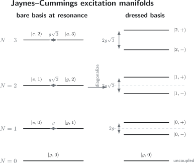
At resonance, each fixed-$\mathcal N=n+1$ bare pair diagonalizes into two equal-weight dressed states. The doublet gap is $2g\sqrt{n+1}$. The vacuum ground state $|g,0\rangle$ forms the one-dimensional $\mathcal N=0$ sector and remains uncoupled.

Exact Dressed Eigenstates

The block Hamiltonian

In the ordered basis $\{|e,n\rangle,|g,n+1\rangle\}$,

$$\begin{gathered} \frac{H_n}{\hbar} = \omega_c \left( n+\frac12 \right)I + \mathcal M_n, \\ \mathcal M_n = \frac12 \begin{pmatrix} \Delta & 2g\sqrt{n+1} \\ 2g\sqrt{n+1} & -\Delta \end{pmatrix}. \end{gathered}$$

Define the manifold-dependent generalized Rabi frequency

$$\Omega_n = \sqrt{ \Delta^2+4g^2(n+1) }.$$

The exact eigenenergies are

$$E_{n,\pm} = \hbar\omega_c \left( n+\frac12 \right) \pm \frac{\hbar\Omega_n}{2}.$$

The uncoupled ground-state energy is

$$E_{g0} = -\frac{\hbar\omega_a}{2}.$$

Mixing angle

Choose $0\leq\theta_n\leq\pi/2$ such that

$$\begin{aligned} \cos(2\theta_n) &= \frac{\Delta}{\Omega_n}, \\ \sin(2\theta_n) &= \frac{2g\sqrt{n+1}}{\Omega_n}. \end{aligned}$$

One continuous eigenstate convention is

$$\begin{aligned} |n,+\rangle &= \cos\theta_n\,|e,n\rangle + \sin\theta_n\,|g,n+1\rangle, \\ |n,-\rangle &= -\sin\theta_n\,|e,n\rangle + \cos\theta_n\,|g,n+1\rangle. \end{aligned}$$

For large positive detuning, the upper state is atom-like and the lower state cavity-like. As $\Delta$ passes through zero, those characters exchange continuously. At resonance,

$$|n,\pm\rangle = \frac{ |e,n\rangle \pm |g,n+1\rangle }{ \sqrt2 },$$

up to independent overall signs. The resonant energy splitting is

$$E_{n,+}-E_{n,-} = 2\hbar g\sqrt{n+1}.$$

Anharmonic dressed ladder

On resonance,

$$\frac{E_{n,\pm}}{\hbar} = \omega_c \left( n+\frac12 \right) \pm g\sqrt{n+1}.$$

The $\sqrt{n+1}$ term makes successive level spacings unequal. This anharmonicity is the origin of number-resolved doublets and enables single-photon nonlinear phenomena such as photon blockade when the linewidths are narrower than the relevant difference between transitions. It weakens at large $n$ because

$$\sqrt{n+1}-\sqrt n \simeq \frac{1}{2\sqrt n}.$$

That shrinking anharmonicity is one route toward the semiclassical limit.

Exact Excitation-Exchange Dynamics

Propagator in one manifold

Subtracting the common block energy leaves the effective two-state Hamiltonian

$$\frac{H_n'}{\hbar} = \frac12 \left[ \Delta\sigma_z + 2g\sqrt{n+1}\,\sigma_x \right].$$

Because $(\mathbf u\mathbin{\cdot}\boldsymbol\sigma)^2=I$ for a unit vector $\mathbf u$, its exponential is immediate:

$$\begin{aligned} U_n(t) ={}& e^{-i\omega_c(n+1/2)t} \widetilde U_n(t), \\ \widetilde U_n(t) ={}& \cos\left(\frac{\Omega_n t}{2}\right)I \\ &- \frac{i}{\Omega_n} \sin\left(\frac{\Omega_n t}{2}\right) K_n, \\ K_n ={}& \Delta\sigma_z + 2g\sqrt{n+1}\,\sigma_x. \end{aligned}$$

Starting from $|e,n\rangle$,

$$\begin{aligned} |\psi_n(t)\rangle ={}& e^{-i\omega_c(n+1/2)t} \Big[ A_n(t)|e,n\rangle \\ &\qquad\qquad + B_n(t)|g,n+1\rangle \Big], \end{aligned}$$

where

$$\begin{aligned} A_n(t) &= \cos\left(\frac{\Omega_n t}{2}\right) - i\frac{\Delta}{\Omega_n} \sin\left(\frac{\Omega_n t}{2}\right), \\ B_n(t) &= - i\frac{2g\sqrt{n+1}}{\Omega_n} \sin\left(\frac{\Omega_n t}{2}\right). \end{aligned}$$

The transfer probability is

$$P_{e,n\to g,n+1}(t) = \frac{ 4g^2(n+1) }{ \Omega_n^2 } \sin^2\left(\frac{\Omega_n t}{2}\right).$$

Detuning has two effects: it raises the oscillation frequency from $2g\sqrt{n+1}$ to $\Omega_n$, while reducing the largest possible transfer to $4g^2(n+1)/\Omega_n^2$. Faster oscillation therefore does not mean better state transfer.

Resonant quantum Rabi oscillations

At $\Delta=0$, remove the common block phase by defining $|\widetilde\psi_n(t)\rangle =e^{i\omega_c(n+1/2)t}|\psi_n(t)\rangle$. Then

$$\begin{aligned} |\widetilde\psi_n(t)\rangle ={}& C_n(t)|e,n\rangle - iS_n(t)|g,n+1\rangle, \\ C_n(t) ={}& \cos\left( g\sqrt{n+1}\,t \right), \\ S_n(t) ={}& \sin\left( g\sqrt{n+1}\,t \right). \end{aligned}$$

Thus

$$\begin{aligned} P_e^{(n)}(t) &= \cos^2\left( g\sqrt{n+1}\,t \right), \\ \langle\sigma_z(t)\rangle_n &= \cos\left( 2g\sqrt{n+1}\,t \right). \end{aligned}$$

The terminology is worth fixing:

• $g\sqrt{n+1}$ is the off-diagonal coupling in angular-frequency units;
• $2g\sqrt{n+1}$ is the resonant dressed splitting and the angular frequency of population inversion;
• $\pi/[2g\sqrt{n+1}]$ is the first complete excitation-transfer time.

For the vacuum, these become $g$, $2g$, and $\pi/(2g)$. At $t=\pi/(4g)$, an initial $|e,0\rangle$ has evolved to a maximally entangled atom-field state,

$$\frac{ |e,0\rangle-i|g,1\rangle }{ \sqrt2 },$$

up to an overall phase. At $t=\pi/(2g)$ the excitation has completely moved to the field and the state is again separable.

Absorption and emission factors

An excited atom in $|e,n\rangle$ emits into a field already containing $n$ quanta with amplitude proportional to $\sqrt{n+1}$. Its squared matrix element contains

$$n+1 = n + 1,$$

which separates naturally into stimulated and vacuum contributions. A ground-state atom absorbs from $|g,n\rangle$ with amplitude $g\sqrt n$; the vacuum cannot supply an excitation for absorption. These facts arise from bosonic ladder operators, not from adding a classical stimulated-emission rule by hand.

Arbitrary Initial Field States

Let the atom begin in $|e\rangle$ and let the field’s photon-number probabilities be

$$P_n = \langle n|\rho_f(0)|n\rangle.$$

Because different number sectors remain orthogonal when the field is traced out, the atomic inversion is

$$\begin{aligned} W(t) &\equiv \langle\sigma_z(t)\rangle \\ &= \sum_{n=0}^{\infty} P_n \frac{\Delta^2}{\Omega_n^2} \\ &\quad+ \sum_{n=0}^{\infty} P_n \frac{4g^2(n+1)}{\Omega_n^2} \cos(\Omega_n t) . \end{aligned}$$

This formula also applies when the initial field has number coherences: $W(t)$ depends only on its diagonal number statistics for this initial atomic state and this observable. Other observables can retain phase information.

Number state

For an initial Fock state $|n_0\rangle$, exactly one frequency contributes:

$$W(t) = \frac{\Delta^2}{\Omega_{n_0}^2} + \frac{4g^2(n_0+1)}{\Omega_{n_0}^2} \cos(\Omega_{n_0}t).$$

In the ideal closed model there is no collapse. A measured decay of this oscillation indicates loss, dephasing, parameter averaging, leakage beyond the model, or an initial number distribution rather than a pure number state.

Coherent state

For $|\alpha\rangle$ with $\bar n=|\alpha|^2$,

$$P_n = e^{-\bar n} \frac{\bar n^n}{n!}.$$

On resonance,

$$W_\alpha(t) = e^{-\bar n} \sum_{n=0}^{\infty} \frac{\bar n^n}{n!} \cos\left( 2g\sqrt{n+1}\,t \right).$$

Every number sector evolves coherently, but each has a slightly different frequency. Their weighted sum first loses visible contrast and later recovers it. This is the Jaynes–Cummings collapse-and-revival effect.

Thermal state

A thermal mode has

$$P_n = \frac{ \bar n^n }{ (1+\bar n)^{n+1} }.$$

Its distribution is broader than a Poisson distribution with the same mean, so many frequencies dephase quickly and do not form the same clean revival sequence. Collapse and revival therefore probe photon-number statistics, not merely mean intensity.

Collapse and Revival

Collapse is unitary dephasing

For $\bar n\gg1$, expand the resonant inversion frequency around the center of the Poisson distribution:

$$\begin{aligned} 2g\sqrt{n+1} \simeq{}& 2g\sqrt{\bar n+1} \\ &+ \frac{g}{\sqrt{\bar n+1}} \left( n-\bar n \right) +\cdots. \end{aligned}$$

The Poisson variance is $\operatorname{Var}(n)=\bar n$. Keeping the linear term gives an early-time Gaussian envelope

$$\begin{gathered} \left| W_\alpha(t) \right|_{\rm env} \approx \exp\left( - \frac{\eta g^2t^2}{2} \right), \\ \eta = \frac{\bar n}{\bar n+1}, \qquad \left| W_\alpha(t) \right|_{\rm env} \simeq e^{-g^2t^2/2}. \end{gathered}$$

If the collapse time is defined by a $1/e$ envelope, then

$$t_{\rm col} \simeq \frac{\sqrt2}{g}.$$

Other quoted collapse times differ because authors use a first-zero, half-contrast, or $1/e$ convention. The scaling and the declared definition matter more than the label.

No environment is required for this collapse. The joint state remains pure. The atom becomes entangled with distinguishable field components, and tracing out the field hides their relative phases from the atomic inversion. This mechanism should not be confused with wavefunction collapse or irreversible decoherence.

Rephasing and revival time

Neighboring number sectors rephase when their accumulated phase difference is approximately $2\pi$. Near $n=\bar n$,

$$\begin{aligned} \Omega_{n+1}-\Omega_n &\simeq \frac{g}{\sqrt{\bar n}}, \\ \left( \Omega_{n+1}-\Omega_n \right)t_{\rm rev} &\simeq 2\pi. \end{aligned}$$

Therefore the first large-$\bar n$ revival occurs near

$$t_{\rm rev} \simeq \frac{ 2\pi\sqrt{\bar n} }{g}.$$

Quadratic and higher terms in the frequency expansion prevent a perfect reconstruction and create fractional-revival structure. The number of rapid Rabi cycles before the first revival grows with $\bar n$.

Semiclassical limit

Write a bright coherent mode as

$$a = \alpha+\delta a.$$

The mean part gives a semiclassical drive with population-inversion frequency $2g|\alpha|=2g\sqrt{\bar n}$, while $\delta a$ carries quantum fluctuations. The relative Poisson width $\sqrt{\operatorname{Var}(n)}/\bar n=1/\sqrt{\bar n}$ vanishes as $\bar n$ grows. Over any fixed number of increasingly rapid Rabi cycles, the evolution approaches a classical-drive result. At sufficiently long times, however, the residual number dependence still produces collapse and revival.

Spectroscopy and Nonlinearity

The same $\sqrt{n+1}$ structure appears in time and frequency domains. On resonance, the first doublet is reached from $|g,0\rangle$ at frequencies

$$\omega_c-g \qquad\text{and}\qquad \omega_c+g.$$

Transitions between higher dressed manifolds involve differences such as

$$\omega_c + g \left( \sqrt{n+1}-\sqrt n \right),$$

with branch-dependent signs and matrix elements. A weak probe can therefore resolve an anharmonic ladder if its linewidth and power broadening are small enough. A strong drive populates several manifolds, dresses the system again, and invalidates a simple two-line interpretation.

Spectral normal-mode splitting can also occur for classical coupled oscillators. The explicitly quantum information is the calibrated $\sqrt{n+1}$ ladder, number-dependent exchange, antibunched output, or another observable that tests excitation quantization.

Applications

Cavity QED

For an atom, ion, molecule, or solid-state emitter in an optical or microwave cavity, $g$ comes from the transition dipole and the vacuum mode field. The ideal model predicts polariton energies and swaps; the experiment also contains cavity decay $\kappa$, emitter decay $\gamma$, pure dephasing, drive ports, and motion. Those physical parameters and their regimes are developed in Cavity QED.

Circuit QED

A superconducting qubit coupled to a microwave resonator realizes the same exchange algebra. Circuit platforms offer strong electrical dipoles and tunable frequencies, but an artificial atom is rarely an exact two-level system. Transmon anharmonicity, higher resonator modes, drive-induced leakage, and counter-rotating corrections must be included when their scales compete with $g$, detuning, or drive amplitude.

In the far-dispersive regime, eliminating exchange gives the familiar state-dependent cavity shift $\chi\simeq g^2/\Delta$. That effective model is a consequence of the Jaynes–Cummings Hamiltonian, but its readout and backaction interpretation belongs to Cavity QED and the open-system circuit-QED map.

Trapped-ion sidebands

For a trapped ion, the oscillator can be a quantized motional mode rather than an electromagnetic field. After moving to a sideband-resolved interaction picture, the red sideband has Jaynes–Cummings form and exchanges an internal excitation with one phonon. The blue sideband has anti-Jaynes–Cummings form and creates or removes both excitations together. The algebra is portable even though the microscopic coupling is different. Trapped-Ion Control derives the spatial-phase coupling, Lamb–Dicke matrix elements, and sideband-selective Hamiltonians.

State transfer and entanglement

A resonant half-swap transfers one excitation between matter and mode; a quarter-swap creates entanglement. Sequences of detuning, swaps, and measurement can synthesize field states or mediate interactions between otherwise separate emitters. Their fidelity depends on pulse timing, occupation-dependent coupling, leakage, and loss, so the ideal propagator is the starting point rather than a complete control model.

Many emitters

Replacing one two-level system by $N$ identical emitters gives the Tavis–Cummings model,

$$\begin{aligned} H_{\rm TC} ={}& \hbar\omega_c a^\dagger a + \hbar\omega_a J_z \\ &+ \hbar g \left( aJ_+ + a^\dagger J_- \right). \end{aligned}$$

Its symmetric one-excitation bright state couples at $g\sqrt N$, while dark states decouple in the ideal identical-emitter limit. This collective enhancement is distinct from the single-emitter factor $\sqrt{n+1}$: $\sqrt N$ counts coherent emitters, whereas $\sqrt{n+1}$ comes from bosonic occupation.

Open and Driven Jaynes–Cummings Systems

A minimal Markovian extension is

$$\begin{aligned} \dot\rho ={}& -\frac{i}{\hbar} \left[ H_{\rm JC}+H_{\rm drv}, \rho \right] + \kappa\mathcal D[a]\rho \\ &+ \gamma\mathcal D[\sigma_-]\rho + \frac{\gamma_\phi}{2} \mathcal D[\sigma_z]\rho. \end{aligned}$$

The closed Hamiltonian still organizes the resonances, but decay moves population between excitation sectors and broadens coherences. A coherent cavity drive also fails to commute with $\mathcal N$, so the driven steady state is not confined to one block. Collapse and revival survive only if the participating number sectors retain coherence until $t_{\rm rev}$; cavity loss is especially damaging at high photon number.

Weak-excitation spectra can be approximated by two damped coupled oscillators. Saturation, photon blockade, multiphoton resonances, and conditional output records require the full density operator or a trajectory description. The open-system cavity-QED map develops that monitored dynamics.

Beyond the Model

The Jaynes–Cummings model should be enlarged when

• $g\sqrt{n+1}$ is no longer small compared with carrier frequencies;
• counter-rotating processes or the Bloch–Siegert shift are resolved;
• several matter levels or oscillator modes participate;
• a drive is strong enough to populate levels outside the truncation;
• spatial motion makes $g$ an operator or a time-dependent quantity;
• material dispersion, diamagnetic terms, or gauge-consistent truncation changes the effective coupling;
• reservoirs have memory or cannot be represented by constant Lindblad rates.

In the ultrastrong-coupling regime, excitation number is not conserved, the ground state is not the bare product $|g,0\rangle$, and the full quantum Rabi or a more microscopic gauge-consistent Hamiltonian is required. The Rabi Model card gives the compact replacement. The AMO Model Index compares this boundary with semiclassical, open two-level, collective, and cavity models.

Computational Notebook

The Cavity QED Simulation Notebook turns the exact manifold results into executable regression tests. It builds the full tensor basis, verifies dressed gaps and vacuum Rabi exchange, measures coherent-state photon-cutoff error, and adds a clearly separated unconditional Lindblad-loss extension.

Common Mistakes

• Calling $g$ the population oscillation frequency. On resonance in manifold $n$, inversion oscillates at $2g\sqrt{n+1}$.
• Using $\sqrt n$ for emission from $|e,n\rangle$. Emission creates a photon and carries $\sqrt{n+1}$; absorption from $|g,n\rangle$ carries $\sqrt n$.
• Forgetting the uncoupled vacuum ground state. $|g,0\rangle$ belongs to a one-dimensional sector, not a dressed doublet.
• Assuming detuning improves transfer because $\Omega_n$ grows. It makes oscillations faster while reducing their amplitude.
• Treating collapse as decoherence. Ideal collapse is reversible unitary dephasing across number sectors.
• Expecting collapse from a number state. A single Fock sector has one Rabi frequency.
• Using $\mathcal N$ conservation after adding a coherent drive or counter-rotating terms. Those terms connect different excitation sectors.
• Inferring field quantization from any doublet. Classical coupled modes also split; the number-dependent ladder is more diagnostic.
• Extending a two-level RWA model into ultrastrong coupling. Matter-level truncation, counter-rotating terms, and gauge consistency must be revisited together.

Exercises

Exercise 1: Which terms conserve excitation number?

For

$$\mathcal N = a^\dagger a+\sigma_+\sigma_-,$$

evaluate its commutator with $a\sigma_+$, $a^\dagger\sigma_-$, $a^\dagger\sigma_+$, and $a+a^\dagger$. Explain which Hamiltonian terms preserve $\mathcal N$ and which preserve only its parity.

Solution

Use

$$\begin{gathered} [a^\dagger a,a]=-a, \\ [ a^\dagger a,a^\dagger ] =a^\dagger, \\ [ \sigma_+\sigma_-,\sigma_+ ] =\sigma_+, \\ [\sigma_+\sigma_-,\sigma_-]=-\sigma_-. \end{gathered}$$

Then

$$\begin{aligned} [\mathcal N,a\sigma_+] &= -a\sigma_++a\sigma_+ =0, \\ [\mathcal N,a^\dagger\sigma_-] &= a^\dagger\sigma_- - a^\dagger\sigma_- =0. \end{aligned}$$

The Jaynes–Cummings exchange terms conserve excitation number. By contrast,

$$\begin{aligned} [\mathcal N,a^\dagger\sigma_+] &= 2a^\dagger\sigma_+, \\ [\mathcal N,a\sigma_-] &= -2a\sigma_-. \end{aligned}$$

Counter-rotating terms change $\mathcal N$ by two. They therefore preserve $(-1)^{\mathcal N}$ even though they do not preserve $\mathcal N$ itself.

Finally,

$$[\mathcal N,a+a^\dagger] = -a+a^\dagger.$$

A coherent cavity drive changes excitation number by one and does not preserve its parity. Thus block diagonalization by $\mathcal N$ applies to the undriven Jaynes–Cummings Hamiltonian, not automatically to driven or full-Rabi dynamics.

Exercise 2: A detuned dressed doublet

Consider manifold $n=3$ with detuning $\Delta=6g$.

1. Find $\Omega_3$ and the two energy shifts relative to the block center.
2. Find $\cos(2\theta_3)$ and $\sin(2\theta_3)$.
3. Find the maximum probability for $|e,3\rangle\to|g,4\rangle$.

Solution

Here $n+1=4$, so

$$\begin{aligned} \Omega_3 &= \sqrt{ (6g)^2+4g^2(4) } \\ &= 2\sqrt{13}\,g. \end{aligned}$$

The eigenenergy shifts from the common center $4.5\hbar\omega_c$ are

$$\pm\frac{\hbar\Omega_3}{2} = \pm\hbar g\sqrt{13}.$$

The mixing-angle functions are

$$\cos(2\theta_3) = \frac{3}{\sqrt{13}}, \qquad \sin(2\theta_3) = \frac{2}{\sqrt{13}}.$$

The largest transfer probability is the prefactor of the sine squared:

$$\begin{aligned} P_{\rm transfer}^{\rm max} &= \frac{ 4g^2(4) }{ (2\sqrt{13}\,g)^2 } \\ &= \frac4{13} \simeq 0.308. \end{aligned}$$

The large detuning makes the eigenstates mostly bare and prevents complete exchange even though $\Omega_3$ exceeds the resonant oscillation frequency.

Exercise 3: Vacuum swap and entanglement

The resonant system starts in $|e,0\rangle$.

1. At what first time is the atom-field entanglement maximal?
2. At what first time is the excitation fully transferred to the field?
3. Find $\langle a^\dagger a\rangle$ and $\langle\sigma_+\sigma_-\rangle$ at both times.

Solution

Ignoring the common phase,

$$|\psi(t)\rangle = \cos(gt)|e,0\rangle - i\sin(gt)|g,1\rangle.$$

Equal Schmidt coefficients first occur when

$$gt=\frac{\pi}{4}, \qquad t_{\rm ent} = \frac{\pi}{4g}.$$

The state is then

$$|\psi(t_{\rm ent})\rangle = \frac{ |e,0\rangle-i|g,1\rangle }{ \sqrt2 },$$

so

$$\langle a^\dagger a\rangle = \langle\sigma_+\sigma_-\rangle = \frac12.$$

Complete transfer first occurs when

$$gt=\frac{\pi}{2}, \qquad t_{\rm swap} = \frac{\pi}{2g}.$$

The state is then $-i|g,1\rangle$, giving

$$\langle a^\dagger a\rangle=1, \qquad \langle\sigma_+\sigma_-\rangle=0.$$

At all times their sum is one, as required by excitation-number conservation.

Exercise 4: Infer coupling from a detuned doublet

In the one-excitation manifold, spectroscopy gives

$$\frac{\Omega_0}{2\pi} = 30\ \mathrm{MHz}, \qquad \frac{\Delta}{2\pi} = 18\ \mathrm{MHz}.$$

Find $g/(2\pi)$, the maximum transfer probability from $|e,0\rangle$, and the time of its first maximum.

Solution

The splitting obeys

$$\Omega_0^2 = \Delta^2+4g^2.$$

Because all quoted values use the same division by $2\pi$,

$$\begin{aligned} 2\frac{g}{2\pi} &= \sqrt{ (30\ \mathrm{MHz})^2 - (18\ \mathrm{MHz})^2 } \\ &= 24\ \mathrm{MHz}. \end{aligned}$$

Therefore

$$\frac{g}{2\pi} = 12\ \mathrm{MHz}.$$

The maximum transfer probability is

$$P_{\rm max} = \frac{4g^2}{\Omega_0^2} = \frac{24^2}{30^2} = 0.64.$$

The first maximum of $\sin^2(\Omega_0t/2)$ occurs at $\Omega_0t=\pi$, hence

$$t_{\rm max} = \frac{\pi}{\Omega_0} = \frac{1}{ 2(30\ \mathrm{MHz}) } \simeq 16.7\ \mathrm{ns}.$$

Exercise 5: Collapse and revival scales

A resonant coherent field has $\bar n=25$ and $g/(2\pi)=50\ \mathrm{kHz}$.

1. Estimate the $1/e$ collapse time.
2. Estimate the first revival time.
3. Estimate the initial central inversion frequency and the number of its periods before the first revival.

Solution

Since $g=2\pi(50\ \mathrm{kHz})$,

$$\begin{aligned} t_{\rm col} &\simeq \frac{\sqrt2}{g} \\ &= \frac{\sqrt2}{ 2\pi(50\ \mathrm{kHz}) } \simeq 4.50\ \mu\mathrm s. \end{aligned}$$

The first revival time is

$$\begin{aligned} t_{\rm rev} &\simeq \frac{2\pi\sqrt{25}}{g} \\ &= \frac5{50\ \mathrm{kHz}} = 100\ \mu\mathrm s. \end{aligned}$$

Near the center of the distribution, the inversion angular frequency is $2g\sqrt{\bar n+1}$, so

$$\frac{ 2g\sqrt{26} }{2\pi} \simeq 510\ \mathrm{kHz}.$$

Its period is about $1.96\ \mu\mathrm s$. The nominal number of central oscillation periods in one revival time is therefore

$$\frac{ 100\ \mu\mathrm s }{ 1.96\ \mu\mathrm s } \simeq 51.$$

The oscillations do not remain visible throughout that interval: they first collapse and then reappear as the number sectors rephase.

Exercise 6: Same mean photon number, different dynamics

Compare two resonant field states with mean occupation $4$:

$$\rho_A=|4\rangle\langle4|, \qquad \rho_B = \frac12|0\rangle\langle0| + \frac12|8\rangle\langle8|.$$

The atom starts excited.

1. Write $W_A(t)$ and $W_B(t)$.
2. Show that their second derivatives at $t=0$ agree.
3. Compare them at $gt=\pi/2$.

Solution

The exact inversions are

$$\begin{aligned} W_A(t) &= \cos\left( 2g\sqrt5\,t \right), \\ W_B(t) &= \frac12\cos(2gt) + \frac12\cos(6gt). \end{aligned}$$

For an arbitrary number distribution,

$$\left. \frac{d^2W}{dt^2} \right|_{t=0} = -4g^2 \langle n+1\rangle.$$

Both states have $\langle n\rangle=4$, so both begin with curvature $-20g^2$. Their later dynamics depends on the full distribution, not just its mean.

At $gt=\pi/2$,

$$\begin{aligned} W_A &= \cos(\pi\sqrt5) \simeq 0.737, \\ W_B &= \frac12\cos\pi + \frac12\cos3\pi = -1. \end{aligned}$$

Identical mean energy and identical short-time curvature do not determine the later atom-field exchange.

Exercise 7: Check the rotating-wave approximation

A nearly resonant circuit has

$$\begin{gathered} \frac{\omega_a}{2\pi} \simeq \frac{\omega_c}{2\pi} = 5.0\ \mathrm{GHz}, \\ \frac{g}{2\pi} = 100\ \mathrm{MHz}. \end{gathered}$$

States up to $n=24$ are appreciably occupied.

1. Evaluate $g\sqrt{n+1}/(\omega_a+\omega_c)$ at the largest occupation.
2. Estimate the counter-rotating frequency shift $g^2/(\omega_a+\omega_c)$.
3. Compare it with $\kappa/(2\pi)=0.5\ \mathrm{MHz}$.

Solution

At $n=24$,

$$\frac{ g\sqrt{n+1} }{ \omega_a+\omega_c } = \frac{ (100\ \mathrm{MHz})(5) }{ 10\,000\ \mathrm{MHz} } = 0.05.$$

This is smaller than one but not parametrically tiny for precision work. The frequency-shift estimate is

$$\frac1{2\pi} \frac{g^2}{\omega_a+\omega_c} \simeq \frac{ (100\ \mathrm{MHz})^2 }{ 10\,000\ \mathrm{MHz} } = 1.0\ \mathrm{MHz}.$$

That estimate is twice the stated cavity linewidth. Even though the rotating-wave model may describe the gross exchange dynamics, a resolved spectroscopic fit should include counter-rotating and multilevel corrections.

Exercise 8: Loss during a vacuum swap

A resonant cavity-QED system has

$$\begin{gathered} \frac{g}{2\pi}=20\ \mathrm{MHz}, \\ \frac{\kappa}{2\pi}=2.0\ \mathrm{MHz}, \qquad \frac{\gamma}{2\pi}=1.0\ \mathrm{MHz}. \end{gathered}$$

Starting from $|e,0\rangle$, estimate the probability of no decay event during the first ideal vacuum swap. Use the ideal populations inside the integrated hazard.

Solution

The ideal swap time is

$$t_{\rm swap} = \frac{\pi}{2g} = \frac{1}{ 4(20\ \mathrm{MHz}) } = 12.5\ \mathrm{ns}.$$

Along the ideal trajectory,

$$\begin{aligned} P_e(t) &= \cos^2(gt), \\ P_c(t) &= \sin^2(gt). \end{aligned}$$

The integrated first-order jump hazard is

$$\begin{aligned} \Lambda &= \int_0^{t_{\rm swap}} \left[ \gamma P_e(t)+\kappa P_c(t) \right]dt \\ &= \frac{\gamma+\kappa}{2} t_{\rm swap}, \end{aligned}$$

because each population averages to one half over a complete transfer. Numerically,

$$\Lambda = \frac{ 2\pi(3.0\ \mathrm{MHz}) }{2} \left( 12.5\ \mathrm{ns} \right) \simeq 0.118.$$

The no-jump estimate is

$$P_{\rm no\ jump} \simeq e^{-\Lambda} \simeq 0.889.$$

This is a useful leading estimate. An exact non-Hermitian or master-equation solution lets unequal losses alter the conditional populations and also accounts for the reduced transfer fidelity after a jump.

References

1. E. T. Jaynes and F. W. Cummings, “Comparison of quantum and semiclassical radiation theories with application to the beam maser,” Proceedings of the IEEE 51, 89–109 (1963).
2. F. W. Cummings, “Stimulated emission of radiation in a single mode,” Physical Review 140, A1051–A1056 (1965).
3. J. H. Eberly, N. B. Narozhny, and J. J. Sanchez-Mondragon, “Periodic spontaneous collapse and revival in a simple quantum model,” Physical Review Letters 44, 1323–1326 (1980).
4. G. Rempe, H. Walther, and N. Klein, “Observation of quantum collapse and revival in a one-atom maser,” Physical Review Letters 58, 353–356 (1987).
5. M. Brune, F. Schmidt-Kaler, A. Maali, J. Dreyer, E. Hagley, J. M. Raimond, and S. Haroche, “Quantum Rabi oscillation: A direct test of field quantization in a cavity,” Physical Review Letters 76, 1800–1803 (1996).
6. B. W. Shore and P. L. Knight, “The Jaynes–Cummings model,” Journal of Modern Optics 40, 1195–1238 (1993).
7. J. M. Raimond, M. Brune, and S. Haroche, “Manipulating quantum entanglement with atoms and photons in a cavity,” Reviews of Modern Physics 73, 565–582 (2001).
8. H. Walther, B. T. H. Varcoe, B.-G. Englert, and T. Becker, “Cavity quantum electrodynamics,” Reports on Progress in Physics 69, 1325–1382 (2006).
9. S. Haroche and J.-M. Raimond, Exploring the Quantum: Atoms, Cavities, and Photons (Oxford University Press, 2006).
10. M. O. Scully and M. S. Zubairy, Quantum Optics (Cambridge University Press, 1997).
11. D. F. Walls and G. J. Milburn, Quantum Optics, 2nd ed. (Springer, 2008).
12. C. C. Gerry and P. L. Knight, Introductory Quantum Optics (Cambridge University Press, 2005).
13. A. Wallraff et al., “Strong coupling of a single photon to a superconducting qubit using circuit quantum electrodynamics,” Nature 431, 162–167 (2004).
14. A. Blais, R.-S. Huang, A. Wallraff, S. M. Girvin, and R. J. Schoelkopf, “Cavity quantum electrodynamics for superconducting electrical circuits: An architecture for quantum computation,” Physical Review A 69, 062320 (2004).
15. A. Blais, A. L. Grimsmo, S. M. Girvin, and A. Wallraff, “Circuit quantum electrodynamics,” Reviews of Modern Physics 93, 025005 (2021).
16. M. Tavis and F. W. Cummings, “Exact solution for an $N$-molecule–radiation-field Hamiltonian,” Physical Review 170, 379–384 (1968).
17. D. Braak, “Integrability of the Rabi model,” Physical Review Letters 107, 100401 (2011).
18. P. Forn-Díaz, L. Lamata, E. Rico, J. Kono, and E. Solano, “Ultrastrong coupling regimes of light–matter interaction,” Reviews of Modern Physics 91, 025005 (2019).