Hanbury Brown–Twiss Interferometry

A Hanbury Brown–Twiss (HBT) experiment measures correlations between intensity records from two detection channels. In a laboratory arrangement, one optical field is usually divided between two detectors and the delay between their events is histogrammed. In astronomical intensity interferometry, two separated collectors observe the same distant source and their intensity fluctuations are correlated electronically.

Both geometries probe second-order coherence. For a stationary field, the central observable is

$$g_{12}^{(2)}(\tau) := \frac{ G_{12}^{(2)}(\tau) }{ I_1I_2 }.$$

Thermal or chaotic light produces excess coincidences over a coherence time: ideal single-mode, single-polarization thermal light has $g^{(2)}(0)=2$. Coherent light has $g^{(2)}(\tau)=1$, while a suitable single-photon source can show a deficit near zero delay. The apparatus is therefore a correlation instrument, not a device tied to one source class.

An HBT result is incomplete unless it identifies the detected modes, delay convention, coincidence or current estimator, accidental baseline, live-time correction, timing response, background policy, and uncertainty model.

Canonical Scope

This page is the canonical home for:

• split-field and separated-collector HBT geometries;
• two-channel coincidence histograms and their normalization;
• thermal bunching as an experimentally resolved feature;
• finite timing resolution, background, dead time, and correlated artifacts in an HBT measurement;
• spatial intensity interferometry, the van Cittert–Zernike relation, and the uniform-disk angular-diameter example;
• the complementary classical random-wave and quantum photodetection interpretations of HBT bunching.

Correlation Functions owns the general normally ordered hierarchy, the definitions of $G^{(1)}$, $G^{(2)}$, and $g^{(2)}$, and the Siegert relation as part of optical coherence theory. Thermal Light owns the thermal state and its photon-number statistics. Photon Counting owns detector POVMs, efficiency calibration, dark counts, dead time, timing jitter, and response matrices.

Beam Splitters owns the two-mode unitary and phase conventions. This page uses that unitary only to show what the HBT splitter does to a correlation. Photon Antibunching owns the nonclassical single-emitter signature and its source-specific failure modes.

Two Experimental Geometries

Split-field HBT

The common laboratory arrangement has five conceptual stages:

1. Select a spatial, spectral, temporal, and polarization mode family.
2. Divide the accepted field between two output channels.
3. Detect each output independently.
4. Preserve detector labels and event times or photocurrents.
5. correlate the two records as a function of relative delay.

A nonpolarizing beam splitter is convenient, but it is not the defining ingredient. A source can illuminate two detector areas directly, or a polarization splitter can route two selected polarizations. What matters is that the channels sample declared field components and produce records whose joint statistics can be compared.

Separated-collector HBT

In spatial intensity interferometry, collectors at positions $\mathbf r_1$ and $\mathbf r_2$ observe one distant source. The projected baseline is

$$\mathbf B_\perp := \mathbf r_{2,\perp} - \mathbf r_{1,\perp}.$$

Each site detects locally. The optical fields need not be physically combined; time-stamped or digitized intensity records can be brought together later. The geometric propagation delay must still be modeled and removed before the same source time is compared.

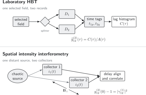
Laboratory HBT estimates a delay-dependent $g_{12}^{(2)}(\tau)$ from two detector records. Spatial intensity interferometry instead varies the projected baseline $\mathbf B_\perp$ and measures the squared first-order coherence of a chaotic source after compensating geometric delay.

Detector reference planes

Every channel should be defined at an optical reference plane before detector loss and electronics. A useful declaration is

$$x_j = (\mathbf r_j,t_j,\lambda_j,\pi_j,u_j),$$

where $\pi_j$ denotes polarization selection and $u_j$ a normalized accepted mode or mode family. Without this declaration, a reduced bunching contrast could come from source statistics, spatial separation, polarization averaging, spectral averaging, or detector response.

Why two detectors?

Two channels turn a same-detector autocorrelation into a cross-correlation. This has practical advantages:

• one detector’s recovery dip does not automatically become a zero-delay anticorrelation in both records;
• independent dark counts contribute an approximately flat accidental baseline;
• channel-specific gains and rates can be monitored separately;
• electrical cross-talk and shared-clock artifacts can be tested with blocked inputs and time shifts.

Two detectors do not remove all artifacts. Optical leakage, electronic cross-talk, common power-supply noise, synchronized gating, or correlated background can still create a false feature.

Amplitude and intensity interferometry

Feature	Amplitude	HBT intensity
primary observable	complex first-order coherence $g^{(1)}$	second-order intensity correlation $g^{(2)}$
optical fields	combined before detection	may be detected independently
phase information	retains a relative optical phase	standard two-channel form returns $
path control	optical-phase stability is central	geometric delay and electronic timing remain central
sensitivity	usually higher for a given optical flux	pays a correlation-statistics penalty
common output	fringe visibility and phase	coincidence excess or current covariance

Intensity interferometry is often more tolerant of optical phase disturbance, but “phase insensitive” does not mean calibration insensitive. Baseline geometry, timing, spectral response, polarization, and detector correlations remain part of the measurement.

The Operational Observable

Normally ordered joint detection

For stationary scalar fields at two detector channels,

$$\begin{aligned} G_{12}^{(2)}(\tau) &= \bigl\langle \hat E_1^{(-)}(t) \hat E_2^{(-)}(t+\tau) \\ &\qquad {} \times \hat E_2^{(+)}(t+\tau) \hat E_1^{(+)}(t) \bigr\rangle. \end{aligned}$$

The normalized function is

$$g_{12}^{(2)}(\tau) = \frac{ G_{12}^{(2)}(\tau) }{ I_1I_2 }, \qquad I_j = \left\langle \hat E_j^{(-)}\hat E_j^{(+)} \right\rangle.$$

Normal ordering is the photodetection ordering. Replacing this expression by an unqualified product of Hermitian intensity operators can introduce vacuum and commutator terms that do not correspond to the same direct-detection record.

Current-fluctuation form

Analog detectors and radio-frequency implementations often correlate photocurrent fluctuations. Define

$$\Delta i_j(t) := i_j(t)-\langle i_j\rangle$$

and

$$C_{12}^{(i)}(\tau) := \left\langle \Delta i_1(t) \Delta i_2(t+\tau) \right\rangle.$$

For linear detectors, negligible cross-talk, and response much faster than the field feature,

$$\frac{ C_{12}^{(i)}(\tau) }{ \langle i_1\rangle \langle i_2\rangle } \propto g_{12}^{(2)}(\tau)-1.$$

The proportionality becomes a calibrated equality only after detector gains, bandwidths, and impulse responses are specified. A digital coincidence histogram and an analog current correlator estimate the same field structure in appropriate limits, but they are not identical raw data products.

Conditional-rate interpretation

Let $\bar R_2$ be the steady rate in channel 2. In an ideal stationary time-tag experiment,

$$R_{2|1}(\tau) = \bar R_2 g_{12}^{(2)}(\tau)$$

is the channel-2 event rate conditioned on a channel-1 event at time zero. Thus:

• $g_{12}^{(2)}(\tau)>1$ means an enhanced conditional rate;
• $g_{12}^{(2)}(\tau)=1$ means the tested event rate equals its steady baseline;
• $g_{12}^{(2)}(\tau)<1$ means a suppressed conditional rate.

This is a statement about an ensemble of records. It does not assign a force between individual photons.

What the Beam Splitter Does

Let $\hat a$ be the accepted source mode and $\hat v$ the unused vacuum input. For one lossless convention,

$$\begin{aligned} \hat b_1 &= \sqrt T\,\hat a + i\sqrt R\,\hat v, \\ \hat b_2 &= i\sqrt R\,\hat a + \sqrt T\,\hat v, \end{aligned}$$

with $R+T=1$. Vacuum in the unused port and normal ordering give

$$\begin{aligned} \langle\hat n_1\rangle &= T\langle\hat n\rangle, \\ \langle\hat n_2\rangle &= R\langle\hat n\rangle. \end{aligned}$$

The cross-channel factorial moment is

$$\left\langle \hat b_1^\dagger \hat b_2^\dagger \hat b_2 \hat b_1 \right\rangle = TR \left\langle \hat a^\dagger \hat a^\dagger \hat a \hat a \right\rangle.$$

Consequently,

$$g_{12,\mathrm{out}}^{(2)}(0) = g_{\mathrm{in}}^{(2)}(0)$$

whenever the denominator is nonzero and the ideal assumptions apply. The splitter routes incident fluctuations to two channels; it does not create the thermal bunching.

The same cancellation holds at nonzero delay for a stationary field when both outputs select the same incident mode family. Unequal filters, polarization projections, nonlinear threshold response, saturation, or correlated background invalidate the simple cancellation.

Thermal Bunching

The Siegert relation in an HBT measurement

For a zero-mean circular complex Gaussian field,

$$g_{12}^{(2)}(\tau) = 1 + \left| g_{12}^{(1)}(\tau) \right|^2.$$

This is the Siegert relation. It connects the measured excess coincidence probability to first-order mutual coherence:

$$g_{12}^{(2)}(\tau)-1 = \left| g_{12}^{(1)}(\tau) \right|^2.$$

At one point, one time, and for one resolved scalar thermal mode,

$$g^{(2)}(0)=2.$$

At delays much longer than the coherence time,

$$g^{(2)}(\tau)\longrightarrow1.$$

The relation requires Gaussian chaotic statistics. A noisy laser, intermittent source, blinking emitter, nonlinear detector, or non-Gaussian field can have $g^{(2)}>1$ without obeying the Siegert relation.

A temporal line-shape example

Suppose a stationary chaotic field has

$$g^{(1)}(\tau) = e^{-i\omega_0\tau} e^{-\gamma|\tau|}.$$

Then

$$g^{(2)}(\tau) = 1 + e^{-2\gamma|\tau|}.$$

The bunching excess has area

$$\mathcal A_c := \int_{-\infty}^{\infty} d\tau\, \left[ g^{(2)}(\tau)-1 \right] = \frac{1}{\gamma}.$$

Peak height and correlation area answer different questions. Timing blur can reduce the observed height while leaving the ideal convolution area unchanged.

Conditional intuition

Chaotic light has fluctuating complex amplitude. An event is more likely when the instantaneous intensity is above average. Conditioning on one event therefore biases the nearby record toward an interval of elevated intensity, and the second event rate is enhanced until the field loses memory.

This language does not imply that an individual count reveals a pre-existing classical intensity in every quantum state. It is an exact intuition for classical Gaussian fields and a useful record-level interpretation of the thermal quantum state.

More than one detected mode

If independent thermal modes have mean detected occupations $\mu_k$, then

$$g^{(2)}(0)-1 = \frac{ \sum_k\mu_k^2 }{ \left( \sum_k\mu_k \right)^2 }.$$

Define

$$M_{\mathrm{eff}} := \frac{ \left( \sum_k\mu_k \right)^2 }{ \sum_k\mu_k^2 }.$$

Then

$$g^{(2)}(0) = 1+\frac{1}{M_{\mathrm{eff}}}.$$

Unresolved polarization, spatial, spectral, or temporal modes reduce the HBT contrast. For two equally weighted independent polarizations, $M_{\mathrm{eff}}=2$ and the ideal unresolved value is $3/2$, not $2$.

Bunching is not a nonclassicality witness

Thermal bunching has a complete classical stochastic-wave account. It is a landmark of higher-order coherence and quantum photodetection, but $g^{(2)}(0)>1$ is not by itself evidence of nonclassical light. A positive Glauber–Sudarshan representation can reproduce it.

The nonclassical statement associated with the following page is different: a stationary classical field under the standard assumptions cannot have a zero-delay value below nearby delayed values. The apparatus may be similar; the inference is not.

Building a Coincidence Histogram

Raw time tags

Let channel 1 record times $t_{1p}$ and channel 2 record times $t_{2q}$. For a lag bin centered at $\tau_k$ with width $\Delta\tau$, define

$$C_k := \sum_{p,q} \mathbf 1_k \left( t_{2q}-t_{1p} \right),$$

where $\mathbf 1_k$ is one when its argument lies in the selected bin and zero otherwise. This definition makes three choices visible:

• which channel starts the delay;
• whether every eligible pair or only a start–stop partner is counted;
• the exact bin edges.

All-pairs correlation is symmetric under channel exchange after reversing delay. A first-stop time-to-amplitude converter produces a waiting-time distribution unless low rates and corrections justify identifying it with an all-pairs correlation.

The accidental baseline

For independent stationary Poisson records with rates $R_1$ and $R_2$, the expected accidental pairs in one bin are approximately

$$A_k \simeq R_1R_2 T_{\mathrm{eff}}(\tau_k) \Delta\tau.$$

Here $T_{\mathrm{eff}}(\tau_k)$ is the overlap of the two channel live-time windows after one record is shifted by $\tau_k$. For uninterrupted acquisition of duration $T_{\mathrm{acq}}$,

$$T_{\mathrm{eff}}(\tau) \simeq T_{\mathrm{acq}}-|\tau|$$

inside the available lag range. The edge correction is negligible only when the plotted delays are small compared with the acquisition duration.

An ideal continuous estimator is

$$\widehat g_{12}^{(2)}(\tau_k) := \frac{C_k}{A_k}.$$

Computing $A_k$ from mean rates is appropriate only when the live time, stationarity, and detector response assumptions hold. Time-shifted records, event mixing between comparable acquisition blocks, or explicit exposure calculation often provide a safer baseline.

Large-delay normalization

If the source is stationary and all physical correlations have decayed, one may normalize by the mean histogram level in a declared far-delay region:

$$\widehat g_{12}^{(2)}(\tau_k) = \frac{ C_k }{ \overline C_{\mathrm{far}} }.$$

This method fails when the selected region contains:

• slow source fluctuations or blinking;
• periodic drive structure;
• afterpulsing or detector recovery;
• clock sidebands or electronic ringing;
• a broad physical correlation tail;
• changing exposure with delay.

The normalization window is part of the result and should be reported.

Pulsed sources

For a source repeated every $T_{\mathrm{rep}}$, the delay histogram often has peaks near

$$\tau=mT_{\mathrm{rep}}, \qquad m\in\mathbb Z.$$

Let $P_m$ be the integrated area of the $m$th peak using identical windows. A common estimator is

$$\widehat g_{\mathrm{pulse}}^{(2)}(0) = \frac{ P_0 }{ \langle P_m\rangle_{m\in\mathcal S} },$$

where $\mathcal S$ is a declared set of nonzero side peaks. The estimator assumes that different pulses are independent, identically prepared, and sampled with the same exposure. Pulse-to-pulse drift, blinking, detector recovery, unequal gates, or a modulated envelope can bias the side-peak baseline.

This pulsed factorial-moment ratio is not automatically the same as an infinitesimal continuous-time value. The gate and pulse mode belong in the definition.

Uncertainty

A histogram bin is not always an independent Poisson variable. One event can contribute to several lag bins, normalization parameters are estimated from the same record, and source drift couples distant delays. Useful uncertainty methods include:

• a likelihood that models the time-tag process and detector response;
• block bootstrap resampling longer than source and detector memory;
• independent acquisition segments with between-segment scatter;
• propagation of rate, background, timing, and baseline calibration uncertainty.

A smooth fitted curve does not replace residual checks or an uncertainty model for the raw counts.

Instrument Response

Linear efficiency cancels from normalized correlation

For independent linear efficiencies $\eta_1$ and $\eta_2$,

$$\begin{aligned} I_{1,\mathrm{det}} &= \eta_1 I_1, \\ I_{2,\mathrm{det}} &= \eta_2 I_2, \end{aligned}$$

and

$$G_{\mathrm{det}}^{(2)} = \eta_1\eta_2 G_{\mathrm{in}}^{(2)}.$$

Therefore the efficiencies cancel in ideal normalized $g^{(2)}$. This invariance does not make efficiency irrelevant. Lower efficiency reduces the number of useful pairs and worsens precision. It also changes the signal fraction relative to fixed dark or background rates.

The cancellation fails for saturation, threshold pileup, state-dependent efficiency, detector memory, or postselection that acts differently on the numerator and denominator.

Independent background dilutes the excess

Let channel $j$ contain signal rate $S_j$ and independent Poisson background rate $B_j$. Define the signal fraction

$$\rho_j := \frac{S_j}{S_j+B_j}.$$

If the signal has correlation $g_{\mathrm s}^{(2)}(\tau)$, then

$$g_{\mathrm{obs}}^{(2)}(\tau)-1 = \rho_1\rho_2 \left[ g_{\mathrm s}^{(2)}(\tau)-1 \right].$$

For equal channels this becomes the familiar squared signal-fraction correction. A background-corrected peak inherits uncertainty from all four rates and from the assumption that the backgrounds are independent and Poissonian.

Correlated stray light, electronic pickup, fluorescence, or clock feedthrough does not obey this formula. Such backgrounds can create a peak rather than merely dilute one.

Timing response convolves the feature

Let $r_{\mathrm{rel}}(\tau)$ be the normalized relative timing-response density of the two channels, including detector jitter and analysis binning. Then the measured excess is approximately

$$h_{\mathrm{obs}}(\tau) = \int d\tau'\, r_{\mathrm{rel}}(\tau-\tau') h_{\mathrm{true}}(\tau'),$$

where

$$h(\tau) := g^{(2)}(\tau)-1.$$

If $r_{\mathrm{rel}}$ is normalized and the integration range is complete,

$$\int d\tau\, h_{\mathrm{obs}}(\tau) = \int d\tau\, h_{\mathrm{true}}(\tau).$$

Thus poor resolution can make a genuine thermal peak shallow while preserving its correlation area. The statement assumes a linear stationary response and no clipping of the fitted delay range.

Timing jitter, timestamp quantization, synchronization drift, and histogram bin width are distinct. A fine digital bin does not undo broad physical jitter.

Dead time, afterpulsing, and cross-talk

Dead time removes events following a detection. In a same-detector autocorrelation it can manufacture a zero-delay dip. A two-detector cross-correlation suppresses that particular artifact, but several effects remain:

• saturation or shared acquisition dead time can couple both channels;
• afterpulses can produce delayed shoulders or peaks;
• optical or electronic cross-talk can produce a narrow zero-delay excess;
• periodic gating and clock leakage can produce a comb;
• pileup can make the response rate dependent.

Blocked-input runs, independent light sources, cable-delay changes, detector swaps, rate scans, and time-shift tests help separate an optical feature from an instrumental one.

Optical bandwidth and timing bandwidth

For chaotic light, narrower optical bandwidth generally lengthens the coherence time and makes a bunching feature easier to resolve. It also reduces the photon rate. For a smooth source spectrum, the photon rate per detected mode decreases roughly in the same proportion that the coherence time increases. Narrow filtering therefore does not provide unlimited signal-to-noise improvement.

The relevant comparison is among:

• optical coherence time;
• detector relative jitter;
• electronic correlation bandwidth;
• histogram bin width;
• source and detector memory times;
• total integration time.

Filtering can still be valuable because it isolates one spectral feature, reduces background, controls modal averaging, and brings the optical correlation within the detector’s timing resolution.

Polarization and mode matching

The two channels need not accept exactly the same polarization or spatial mode. For vector fields, the HBT numerator contains the relevant polarization projections of the coherence matrix. Orthogonal, statistically independent polarizations have no mutual bunching excess. Partial overlap gives an intermediate value.

A useful calibration varies the analyzer angle or spatial overlap. A peak that does not follow the predicted optical projection may be technical intensity noise or electronic cross-talk.

Spatial Intensity Interferometry

Geometric delay

For baseline $\mathbf B=\mathbf r_2-\mathbf r_1$ and source direction $\mathbf s$, one common geometric-delay convention is

$$\tau_{\mathrm g} = \frac{ \mathbf B\cdot\mathbf s }{c}.$$

The sign depends on which detector defines positive delay. A spatial HBT analysis correlates after applying the declared geometric delay, clock offsets, cable delays, and detector latency. Earth rotation changes both the projected baseline and the delay during a stellar observation.

From bunching to mutual coherence

For quasi-monochromatic, spatially incoherent, Gaussian chaotic radiation, the equal-source-time Siegert relation gives

$$g_{12}^{(2)}(0)-1 = \left| \gamma_{12}^{(1)} \right|^2.$$

The quantity $\gamma_{12}^{(1)}$ is the normalized mutual coherence of the field at the two collectors. The experiment therefore measures a squared visibility even though no optical fringe is formed between the collectors.

Finite timing resolution, unresolved polarization, optical bandwidth, and other accepted modes multiply or average the ideal contrast. A practical fit often has the form

$$g_{12}^{(2)}(0)-1 = \beta \left| \gamma_{12}^{(1)} \right|^2,$$

where $\beta$ is a calibrated contrast factor. It is not legitimate to set $\beta=1$ merely because the source is thermal.

The van Cittert–Zernike relation

Let $I_{\mathrm s}(\boldsymbol\theta)$ be the angular brightness distribution of a distant, spatially incoherent source over small sky angle $\boldsymbol\theta$. Define the dimensionless spatial frequency

$$\mathbf u := \frac{\mathbf B_\perp}{\lambda}.$$

The far-field coherence is the normalized Fourier transform

$$\gamma^{(1)}(\mathbf u) = \frac{ \widetilde I_{\mathrm s}(\mathbf u) }{ \widetilde I_{\mathrm s}(\mathbf 0) },$$

with

$$\widetilde I_{\mathrm s}(\mathbf u) := \int d^2\theta\, I_{\mathrm s}(\boldsymbol\theta) e^{-2\pi i\mathbf u\cdot\boldsymbol\theta}.$$

This is the van Cittert–Zernike relation under its usual far-field, quasi-monochromatic, and spatial-incoherence assumptions. The Fourier convention and projected baseline must be stated together.

Fourier Transform develops the transform independently of this optical application.

Uniform circular disk

For a uniformly bright circular disk of angular diameter $\theta_{\mathrm d}$,

$$\gamma^{(1)}(B_\perp) = \frac{2J_1(x)}{x},$$

where

$$x := \frac{ \pi B_\perp\theta_{\mathrm d} }{\lambda}.$$

The measured baseline curve is

$$g^{(2)}(B_\perp,0)-1 = \beta \left[ \frac{2J_1(x)}{x} \right]^2.$$

The first zero of $J_1$ is near $x=3.8317$, so

$$B_0 \simeq \frac{ 1.22\,\lambda }{ \theta_{\mathrm d} }.$$

This estimate exposes the angular-resolution scale. A real star is not usually a uniform disk: limb darkening, rotation, companions, winds, spectral lines, and wavelength-dependent photospheric structure alter the visibility curve. Bessel Functions gives the mathematical properties of $J_1$.

Broadband and projected-baseline fitting

A trustworthy angular-diameter fit forward models:

• the time-dependent projected baseline in the sky plane;
• the geometric delay and clock calibration;
• the full spectral transmission and detector response;
• polarization and modal contrast;
• the stellar brightness model, including limb darkening when relevant;
• zero-baseline or reference-source calibration;
• correlated uncertainty between delay and baseline bins.

For broad spectral response, the measured correlation is a weighted average of wavelength-dependent squared coherence. Replacing the band by one “effective wavelength” is an approximation whose error should be checked.

What information is lost?

Standard two-detector HBT measures

$$\left| \gamma^{(1)}(\mathbf u) \right|^2,$$

not the complex phase of $\gamma^{(1)}$. Consequently, source translation multiplies the Fourier transform by a phase but leaves the measured quantity unchanged. Mirror-related or otherwise phase-ambiguous brightness distributions can also share the same squared visibility.

An angular diameter can be inferred by fitting a constrained source model. General image reconstruction is a phase-retrieval problem and needs broad baseline coverage, priors, or higher-order information. A two-detector baseline curve alone is not a unique image.

Classical Wave Interpretation

Let $E_1$ and $E_2$ be zero-mean circular complex Gaussian field amplitudes. The detected intensities are

$$I_j = E_j^*E_j.$$

Gaussian moment factorization gives

$$\begin{aligned} \langle I_1I_2\rangle ={}& \langle I_1\rangle \langle I_2\rangle \\ &+ \left| \langle E_1^*E_2\rangle \right|^2. \end{aligned}$$

After normalization,

$$g_{12}^{(2)} = 1 + \left| g_{12}^{(1)} \right|^2.$$

The interpretation is intensity fluctuation correlation. Two detectors sample the same random wave pattern to the extent quantified by mutual coherence. When one channel sees an above-average fluctuation, the other is more likely to do so as well.

This derivation explains why thermal HBT bunching does not require photon interactions and is not uniquely quantum. It also displays the assumptions: zero mean, Gaussian statistics, linear intensity detection, and the chosen mode projections.

Quantum Photodetection Interpretation

Quantum theory assigns the coincidence rate to the normally ordered expectation

$$G_{12}^{(2)} = \operatorname{Tr} \left[ \rho\, \hat E_1^{(-)} \hat E_2^{(-)} \hat E_2^{(+)} \hat E_1^{(+)} \right].$$

For chaotic radiation from many independent source elements, two detections can arise through alternatives that exchange which source contribution reaches which detector. When those alternatives are indistinguishable, their amplitudes interfere. The exchange term is positive for the bosonic optical field and produces the same mutual-coherence contribution found in the Gaussian-wave calculation.

The operator account is more general than the classical one:

• it defines direct detection for states without a positive classical probability representation;
• it distinguishes normal, symmetric, and time ordering;
• it predicts coherent, thermal, Fock, squeezed, and emitter-field correlations in one framework;
• it connects the measured record to a density operator and detector POVM.

For thermal Gaussian light, the classical and quantum predictions agree. Calling one description “the real cause” adds no experimentally testable content within their shared domain.

Not evidence that photons attract

Bunching does not mean that photons exert an attractive force. The field propagates linearly in the ideal HBT experiment. The excess is a correlation of a prepared state and selected modes, revealed by joint detection.

Likewise, the phrase “photon arrival time” is shorthand for a detector event time. Propagation, absorption, carrier generation, thresholding, and timestamp assignment lie between the field and the stored record.

Historical Arc

Hanbury Brown and Twiss first developed intensity interferometry for radio astronomy. Their 1954 instrument correlated independently detected intensity fluctuations rather than preserving radio-frequency phase across the baseline.

In 1956 they reported an optical laboratory experiment in which light from one source was divided between two photodetectors and the output fluctuations were correlated. The title’s phrase “coherent beams” used the coherence language of that period; it should not be read as a claim that the source was an ideal Glauber coherent state.

Later in 1956 they tested a separated-collector optical intensity interferometer on Sirius. A detailed series in the Proceedings of the Royal Society A developed the theory, laboratory tests, astronomical application, and Sirius measurement. The later Narrabri Stellar Intensity Interferometer reported angular diameters for 32 stars.

Glauber’s 1963 photodetection theory placed these measurements within the normally ordered hierarchy of optical coherence. HBT methods now span astronomy, laboratory quantum optics, source characterization, and correlations of other identical particles, although those extensions require their own source and detector models.

Interpreting a Measured Feature

Observation	Possible physical meaning	Essential checks
peak near zero delay	thermal bunching or another positive source correlation	timing response, background, cross-talk, mode count
flat value near one	coherent-like statistics, washed-out feature, or uncorrelated channels	resolution, contrast calibration, rate, overlap
dip near zero delay	source antibunching or detector recovery	separate detectors, dead time, background, stationarity
broad excess	slow source noise, blinking, diffusion, or technical power fluctuations	acquisition segments, spectrum, power stability
periodic peaks	pulsed source, gating, clocks, or afterpulsing	repetition period, cable delays, blocked-input run
baseline-dependent excess	spatial mutual coherence	projected baseline, delay tracking, source model, wavelength

The same visual shape can have different origins. Interpretation must follow from a forward model and controls, not from resemblance to a textbook plot.

Reporting Checklist

1. Source and mode. State spectrum, polarization, spatial acceptance, temporal gate, and stationarity assumptions.
2. Geometry. Give splitter ratio or collector coordinates, projected baseline, and delay-sign convention.
3. Detectors. Report efficiencies, rates, timing responses, dead times, afterpulsing, saturation limits, and cross-talk tests.
4. Raw record. Identify time tags, digitized currents, gates, acquisition duration, and live-time gaps.
5. Estimator. Define bin edges, pair rule, accidental baseline, side-peak set, and edge correction.
6. Corrections. Separate raw, background-corrected, deconvolved, and inferred quantities.
7. Fit. State the correlation model, timing convolution, wavelength weighting, and nuisance parameters.
8. Uncertainty. Include baseline, background, calibration, model, and finite-record uncertainty.
9. Controls. Show blocked-input, time-shift, detector-swap, rate-scan, or independent-source checks as appropriate.

Common Mistakes

Saying the splitter creates bunching

An ideal splitter routes the incident factorial moment to two outputs. Normalized $g^{(2)}$ is unchanged under the assumptions derived above.

Treating every peak as thermal

Classical technical noise, blinking, afterpulsing, cross-talk, and periodic electronics can all produce positive correlations. Thermal attribution requires mode, line-shape, scaling, and control evidence.

Calling a reduced peak nonthermal without modeling resolution

An ideal one-mode thermal source can yield an observed value far below two when the coherence time is shorter than detector jitter or the selected bin. Unresolved modes and background reduce it further.

Normalizing to a contaminated delay window

A far-delay region is a baseline only if physical and instrumental correlations have decayed and exposure is comparable.

Ignoring event-pair conventions

All-pairs, first-stop, gated, and pulsed peak-area analyses estimate different objects unless a limiting argument connects them.

Confusing HBT with Hong–Ou–Mandel interference

Standard HBT divides one field or compares two views of one chaotic source and measures intensity correlation. Hong–Ou–Mandel interference injects two one-photon wave packets into two input ports and tests their indistinguishable two-particle alternatives. The optical hardware can look similar, but the state preparation and observable differ.

Claiming complete imaging from squared visibility

Two-detector spatial HBT loses the ordinary Fourier phase. A fitted diameter is a model-dependent inference, not an unconstrained image.

Practical Workflow

1. Specify the field modes and detector reference planes.
2. Choose continuous, pulsed, or spatial-baseline correlation.
3. Preserve detector labels, raw time tags or currents, and live-time masks.
4. Calibrate delay, jitter, rates, background, dead time, and cross-talk.
5. Construct raw pair counts before background or response correction.
6. Build the accidental baseline from actual exposure and declared controls.
7. Forward model timing response, modal contrast, and spatial or temporal coherence.
8. Fit raw and corrected representations separately.
9. Test stability across binning, normalization windows, rates, and acquisition segments.
10. Report the estimator and uncertainty budget with the quoted $g^{(2)}$ or angular diameter.

Connections

• Correlation Functions for $G^{(1)}$, $G^{(2)}$, the Siegert relation, classical bounds, and higher-order coherence.
• Photon Counting for detector POVMs, efficiency, background, dead time, timing response, and response matrices.
• Thermal Light for the Gibbs state, Bose–Einstein number statistics, multimode thermal light, and the source-side bunching derivation.
• Photon Number States for the ideal single-photon splitter test and its distinction from brightness or indistinguishability.
• Beam Splitters for the full two-mode unitary and phase conventions.
• Interferometers for first-order amplitude interferometry and phase estimation.
• Single-Particle Detection for coincidence logic in the broader experimental context.
• AMO Experiment Index for an evidence-level comparison with Hong–Ou–Mandel interference and other landmark AMO measurements.

Exercises

1. The splitter does not change normalized bunching

A source mode $\hat a$ enters a lossless splitter with vacuum in the other input. The outputs have power fractions $T$ and $R$. Show that the cross-channel zero-delay correlation equals the source correlation.

Solution

With vacuum in the unused port, normally ordered moments containing a nontrivial vacuum operator vanish. The mean output occupations are

$$\begin{aligned} \langle\hat n_1\rangle &= T\langle\hat n\rangle, \\ \langle\hat n_2\rangle &= R\langle\hat n\rangle. \end{aligned}$$

The coincidence numerator is

$$\left\langle \hat b_1^\dagger \hat b_2^\dagger \hat b_2 \hat b_1 \right\rangle = TR \left\langle \hat a^\dagger \hat a^\dagger \hat a \hat a \right\rangle.$$

Therefore

$$\begin{aligned} g_{12,\mathrm{out}}^{(2)}(0) &= \frac{ TR \langle \hat a^\dagger\hat a^\dagger\hat a\hat a \rangle }{ TR\langle\hat n\rangle^2 } \\ &= g_{\mathrm{in}}^{(2)}(0). \end{aligned}$$

The routing factors cancel. The equality assumes linear detection, a vacuum unused input, and nonzero mean source intensity.

2. Bunching diluted by a finite delay bin

An ideal chaotic field has

$$g^{(2)}(\tau) = 1+e^{-2\gamma|\tau|}.$$

A histogram reports the average over a top-hat zero-delay bin of width $\Delta$. Find the reported value and its limits for $\gamma\Delta\ll1$ and $\gamma\Delta\gg1$.

Solution

The averaged excess is

$$\overline h_0 = \frac{1}{\Delta} \int_{-\Delta/2}^{\Delta/2} d\tau\, e^{-2\gamma|\tau|}.$$

Using symmetry,

$$\begin{aligned} \overline h_0 &= \frac{2}{\Delta} \int_0^{\Delta/2} d\tau\, e^{-2\gamma\tau} \\ &= \frac{ 1-e^{-\gamma\Delta} }{ \gamma\Delta }. \end{aligned}$$

Hence

$$\overline g_0^{(2)} = 1+ \frac{ 1-e^{-\gamma\Delta} }{ \gamma\Delta }.$$

For a well-resolved peak,

$$\overline g_0^{(2)} = 2-\frac{\gamma\Delta}{2} + O\!\left((\gamma\Delta)^2\right).$$

For a bin much wider than the coherence time,

$$\overline g_0^{(2)} \simeq 1+\frac{1}{\gamma\Delta}.$$

The source remains single-mode thermal even though the observed peak tends toward one as the bin widens.

3. Unequally weighted thermal modes

Three independent thermal modes contribute mean detected rates in the ratio $4:2:1$. Find $M_{\mathrm{eff}}$ and the ideal zero-delay HBT value.

Solution

The effective mode number is

$$M_{\mathrm{eff}} = \frac{(4+2+1)^2}{4^2+2^2+1^2} = \frac{49}{21} = \frac{7}{3}.$$

Therefore

$$\begin{aligned} g^{(2)}(0) &= 1+\frac{1}{M_{\mathrm{eff}}} \\ &= 1+\frac{3}{7} \\ &= \frac{10}{7}. \end{aligned}$$

The value is about $1.43$. Counting modes without their weights would give the wrong contrast.

4. Asymmetric background dilution

An ideal thermal signal has $g_{\mathrm s}^{(2)}(0)=2$. Channel 1 has signal and background rates

$$S_1=60\,\mathrm{kHz}, \qquad B_1=10\,\mathrm{kHz},$$

while channel 2 has

$$S_2=45\,\mathrm{kHz}, \qquad B_2=15\,\mathrm{kHz}.$$

Assuming independent Poisson backgrounds, predict the raw zero-delay value.

Solution

The signal fractions are

$$\rho_1 = \frac{60}{70} = \frac67$$

and

$$\rho_2 = \frac{45}{60} = \frac34.$$

The observed excess is

$$\begin{aligned} g_{\mathrm{obs}}^{(2)}(0)-1 &= \rho_1\rho_2 \left[ g_{\mathrm s}^{(2)}(0)-1 \right] \\ &= \frac67\frac34 \\ &= \frac{9}{14}. \end{aligned}$$

Thus

$$g_{\mathrm{obs}}^{(2)}(0) = \frac{23}{14} \simeq 1.64.$$

A raw value below two is expected even before timing blur or multimode averaging.

5. Continuous-time accidental normalization

Two stationary channels have rates

$$\begin{aligned} R_1&=4.0\times10^4\,\mathrm{s}^{-1}, \\ R_2&=3.0\times10^4\,\mathrm{s}^{-1}. \end{aligned}$$

They are recorded for $100\,\mathrm{s}$ with no gaps. A central lag bin has width $1.0\,\mathrm{ns}$ and contains 150 pairs. Estimate its accidental baseline and normalized correlation. Neglect edge effects.

Solution

The independent-record baseline is

$$\begin{aligned} R_1R_2 &= 1.2\times10^9\,\mathrm{s}^{-2}, \\ T_{\mathrm{acq}}\Delta\tau &= 1.0\times10^{-7}\,\mathrm{s}^{2}, \\ A_0 &= R_1R_2T_{\mathrm{acq}}\Delta\tau =120. \end{aligned}$$

The normalized estimate is

$$\widehat g^{(2)}(0) = \frac{150}{120} = 1.25.$$

A naive counting-only standard error would be approximately

$$\frac{\sqrt{150}}{120} \simeq 0.10,$$

but a complete uncertainty includes the estimated rates, baseline exposure, shared-event covariance, and any background or timing correction.

6. Angular diameter from the first visibility zero

At wavelength $\lambda=443\,\mathrm{nm}$, a uniform-disk fit places the first zero of the HBT baseline curve at $B_0=17.7\,\mathrm m$. Estimate the angular diameter in radians and milliarcseconds.

Solution

For a uniform disk,

$$\theta_{\mathrm d} \simeq \frac{1.22\,\lambda}{B_0}.$$

Substitution gives

$$\begin{aligned} \theta_{\mathrm d} &\simeq \frac{ 1.22(443\times10^{-9}\,\mathrm m) }{ 17.7\,\mathrm m } \\ &\simeq 3.05\times10^{-8}\,\mathrm{rad}. \end{aligned}$$

Using

$$1\,\mathrm{rad} \simeq 2.06265\times10^8\,\mathrm{mas},$$

one obtains

$$\theta_{\mathrm d} \simeq 6.3\,\mathrm{mas}.$$

This is a uniform-disk diameter. A limb-darkened diameter requires an additional source model and bandpass treatment.

7. Why standard two-detector HBT loses source position

Let a sky brightness distribution be translated by $\boldsymbol\theta_0$:

$$I'_{\mathrm s}(\boldsymbol\theta) = I_{\mathrm s} \left( \boldsymbol\theta-\boldsymbol\theta_0 \right).$$

Show that the standard HBT baseline observable is unchanged.

Solution

Apply the shift theorem to the source Fourier transform:

$$\widetilde I'_{\mathrm s}(\mathbf u) = e^{-2\pi i\mathbf u\cdot\boldsymbol\theta_0} \widetilde I_{\mathrm s}(\mathbf u).$$

Normalization at $\mathbf u=\mathbf0$ is unchanged, so

$$\gamma'^{(1)}(\mathbf u) = e^{-2\pi i\mathbf u\cdot\boldsymbol\theta_0} \gamma^{(1)}(\mathbf u).$$

Taking the squared modulus removes the translation phase:

$$\left| \gamma'^{(1)}(\mathbf u) \right|^2 = \left| \gamma^{(1)}(\mathbf u) \right|^2.$$

Standard two-detector HBT therefore cannot determine an absolute image centroid from squared visibility alone. This is one concrete form of the phase-retrieval ambiguity.

8. Derive thermal bunching from Gaussian waves

Let $E_1$ and $E_2$ be zero-mean circular complex Gaussian field amplitudes. Use Gaussian moment factorization to derive the two-channel Siegert relation. Explain why the result is not a nonclassicality witness.

Solution

The intensity product is

$$I_1I_2 = E_1^*E_1E_2^*E_2.$$

Gaussian factorization pairs the four amplitudes. Circularity makes the anomalous pairings

$$\langle E_1E_2\rangle \quad\text{and}\quad \langle E_1^*E_2^*\rangle$$

vanish. The remaining terms give

$$\begin{aligned} \langle I_1I_2\rangle ={}& \langle E_1^*E_1\rangle \langle E_2^*E_2\rangle \\ &+ \langle E_1^*E_2\rangle \langle E_1E_2^*\rangle. \end{aligned}$$

Because the last two factors are complex conjugates,

$$\langle I_1I_2\rangle = \langle I_1\rangle \langle I_2\rangle + \left| \langle E_1^*E_2\rangle \right|^2.$$

Divide by $\langle I_1\rangle\langle I_2\rangle$:

$$g_{12}^{(2)} = 1+ \left| g_{12}^{(1)} \right|^2.$$

The derivation used a classical random field with a positive probability distribution. Thermal bunching is therefore compatible with classical wave statistics. Quantum photodetection reproduces and generalizes the result, but the inequality $g^{(2)}>1$ alone does not certify nonclassical light.

References

1. R. Hanbury Brown and R. Q. Twiss, “A New Type of Interferometer for Use in Radio Astronomy,” Philosophical Magazine 45, 663–682 (1954), doi:10.1080/14786440708520475.
2. R. Hanbury Brown and R. Q. Twiss, “Correlation between Photons in Two Coherent Beams of Light,” Nature 177, 27–29 (1956), doi:10.1038/177027a0.
3. R. Hanbury Brown and R. Q. Twiss, “A Test of a New Type of Stellar Interferometer on Sirius,” Nature 178, 1046–1048 (1956), doi:10.1038/1781046a0.
4. R. Hanbury Brown and R. Q. Twiss, “Interferometry of the Intensity Fluctuations in Light. I. Basic Theory: The Correlation between Photons in Coherent Beams of Radiation,” Proceedings of the Royal Society A 242, 300–324 (1957), doi:10.1098/rspa.1957.0177.
5. R. Hanbury Brown and R. Q. Twiss, “Interferometry of the Intensity Fluctuations in Light. II. An Experimental Test of the Theory for Partially Coherent Light,” Proceedings of the Royal Society A 243, 291–319 (1958), doi:10.1098/rspa.1958.0001.
6. P. H. van Cittert, “Die wahrscheinliche Schwingungsverteilung in einer von einer Lichtquelle direkt oder mittels einer Linse beleuchteten Ebene,” Physica 1, 201–210 (1934), doi:10.1016/S0031-8914(34)90026-4.
7. F. Zernike, “The Concept of Degree of Coherence and Its Application to Optical Problems,” Physica 5, 785–795 (1938), doi:10.1016/S0031-8914(38)80203-2.
8. R. J. Glauber, “The Quantum Theory of Optical Coherence,” Physical Review 130, 2529–2539 (1963), doi:10.1103/PhysRev.130.2529.
9. B. L. Morgan and L. Mandel, “Measurement of Photon Bunching in a Thermal Light Beam,” Physical Review Letters 16, 1012–1015 (1966), doi:10.1103/PhysRevLett.16.1012.
10. R. Hanbury Brown, J. Davis, and L. R. Allen, “The Angular Diameters of 32 Stars,” Monthly Notices of the Royal Astronomical Society 167, 121–136 (1974), doi:10.1093/mnras/167.1.121.
11. A. U. Abeysekara et al., “Demonstration of Stellar Intensity Interferometry with the Four VERITAS Telescopes,” Nature Astronomy 4, 1164–1169 (2020), doi:10.1038/s41550-020-1143-y.
12. G. Baym, “The Physics of Hanbury Brown–Twiss Intensity Interferometry: From Stars to Nuclear Collisions,” Acta Physica Polonica B 29, 1839–1884 (1998), arXiv:nucl-th/9804026.
13. L. Mandel and E. Wolf, Optical Coherence and Quantum Optics, Cambridge University Press (1995), doi:10.1017/CBO9781139644105.
14. J. W. Goodman, Statistical Optics, 2nd ed., Wiley (2015).
15. R. Hanbury Brown, The Intensity Interferometer: Its Application to Astronomy, Taylor & Francis (1974).
16. R. Loudon, The Quantum Theory of Light, 3rd ed., Oxford University Press (2000).