Photon Counting

Photon counting converts an optical field into discrete classical outcomes: an integer per acquisition gate, an off/click result, a set of time tags, or a spatial pattern of events. The word photon in the name does not make the record identical to the incident photon number. Between a declared optical reference plane and the stored data lie propagation loss, mode mismatch, conversion efficiency, thresholding, recovery dynamics, electronics, and data selection.

A quantitative photon-counting result therefore requires three distinct objects:

1. the quantum state of specified incident modes;
2. a detector POVM or response model at a specified reference plane;
3. a statistical model for the recorded outcomes and its uncertainties.

This separation prevents two common errors. A click is not automatically a nondestructive report that one localized photon existed before measurement, and an efficiency-corrected histogram is not raw data. Photon counting is an absorptive quantum measurement whose meaning is fixed by a calibrated model.

Canonical Scope

This page is the canonical home for optical photon counting as a detector response problem:

• the Glauber–Kelley–Kleiner photodetection formula;
• photon-number-resolving, threshold, multiplexed, and time-tagged outcomes;
• Bernoulli loss and efficiency-dependent counting statistics;
• dark counts, background, dead time, timing jitter, afterpulsing, and saturation;
• optical counting POVMs and response matrices;
• detector calibration, tomography, unfolding, and uncertainty reporting.

Photon Number States owns the prepared-state number distribution, source quality, heralding, and phase properties. Photon Counting in the open-systems volume owns conditional intensities, time-tag records, no-click information, and stochastic counting processes. Quantum Jump Trajectories owns the conditioned state update. POVMs owns the abstract measurement formalism, and Measurement Tomography owns general reconstruction theory. The present page specializes those tools to calibrated optical detectors. Photonic Qubits places those detector models inside destructive readout, Bell analysis, fusion, feed-forward, and accepted-event accounting.

What Is Being Counted?

Declare a reference plane

Let the detector reference plane be the optical plane at which an incident state is defined. All losses upstream of that plane belong to state preparation or propagation. All losses downstream belong to the detector response. Moving the plane changes the numerical efficiency but not any prediction if the state and response are transformed consistently.

This bookkeeping matters when efficiencies from different experiments are compared. An intrinsic absorption probability, a packaged detector efficiency, and a system detection efficiency including collection optics are different quantities.

Declare modes and gates

A photon number is an occupation number of a mode. A detector instead couples to a weighted family of spatial, spectral, polarization, and temporal modes. For a pulsed experiment, a gate $g$ might refer to one laser period and the incident probabilities are

$$P_n^{(g)} = \langle n|\rho_g|n\rangle.$$

For a continuous field, a time interval $[t_0,t_0+T]$ defines an exposure, but the events need not correspond to occupation of one normalized temporal mode. A spectral filter, fiber, aperture, polarization analyzer, detector area, and timing gate jointly define what reaches the active element.

Mode mismatch can often be represented as loss only when unmatched modes are discarded and do not themselves produce background. If several accepted modes contribute, their occupations and correlations must be included explicitly.

Four common outcome spaces

• A photon-number-resolving detector returns an integer $k=0,1,2,\ldots$ over a declared gate.
• A threshold detector returns off or click. It cannot distinguish one registered quantum from several.
• A time-tagging detector returns event times and often detector-channel labels. Binning those tags produces counts but discards timing information.
• A spatially resolving detector returns pixel labels or an event image, sometimes with time and energy information as well.

The appropriate POVM is indexed by the actual stored outcomes. Relabeling a threshold click as “one photon” silently invents number resolution that the instrument does not possess.

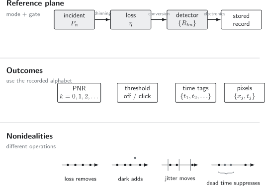
Photon counting is a chain from a declared incident mode and reference plane to a calibrated response and finally a stored record. Loss thins events, dark counts add events, timing jitter moves them, and dead time removes nearby events; these operations are not interchangeable.

Microscopic Photodetection

Positive-frequency field

Write the detected electric field as

$$\begin{aligned} \mathbf E(\mathbf r,t) &= \mathbf E^{(+)}(\mathbf r,t) + \mathbf E^{(-)}(\mathbf r,t), \\ \mathbf E^{(-)} &= \left(\mathbf E^{(+)}\right)^\dagger. \end{aligned}$$

In the usual electric-dipole and rotating-wave approximations, excitation of an initially unexcited absorber contains $\mathbf E^{(+)}$, which annihilates an optical excitation. Summing over unresolved detector final states gives an ideal first-order count rate proportional to

$$R(t) \propto \left\langle \mathbf E^{(-)}(\mathbf r,t) \mathbin{\cdot} \mathbf E^{(+)}(\mathbf r,t) \right\rangle.$$

Normal ordering is physical here: an ideal absorber responds to energy absorption, not directly to the symmetrized vacuum variance. Detector bandwidth, polarization response, and spatial acceptance are suppressed in this compact expression.

Integrated exposure

For a gate $G$, define a dimensionless positive exposure operator

$$\begin{aligned} \hat W_G ={}& \int_G dt \int_G dt'\, \\ &\hat{\mathbf E}^{(-)}(t) \mathbin{\cdot} \boldsymbol{\Gamma}(t,t') \mathbin{\cdot} \hat{\mathbf E}^{(+)}(t'). \end{aligned}$$

The kernel $\boldsymbol{\Gamma}$ contains the detector response and normalization. In a broadband detector with response short compared with the field dynamics, it becomes approximately local in time. For one perfectly matched mode under linear loss,

$$\hat W_G = \eta\hat n.$$

This reduction is useful, but it is not the definition of photodetection. It assumes that one mode and one scalar efficiency adequately describe the full coupling.

Glauber–Kelley–Kleiner formula

For an ideal linear counter with no dead time or saturation, the probability of $m$ photoevents in the gate is

$$p_m = \left\langle : \frac{\hat W_G^m}{m!} e^{-\hat W_G} : \right\rangle.$$

The colons denote normal ordering. The associated probability-generating function is

$$G_M(z) = \sum_{m=0}^{\infty}p_m z^m = \left\langle : e^{-(1-z)\hat W_G} : \right\rangle.$$

For a coherent field, normal-ordered moments factorize and the counts are Poisson distributed. For a fluctuating classical intensity, the result is a mixture of Poisson distributions. Nonclassical states can yield statistics that no positive mixture of classical intensities reproduces.

The formula relies on an absorber model, linear response, the relevant rotating-wave and bandwidth approximations, and negligible detector memory during the gate. Recovery, afterpulsing, and saturation require a detector state or a phenomenological response beyond $\hat W_G$.

Ideal Counting POVMs

Perfect number resolution

For one mode and an ideal destructive number measurement,

$$\Pi_n^{\mathrm{PNR}} = |n\rangle\langle n|, \qquad \sum_{n=0}^{\infty}\Pi_n^{\mathrm{PNR}} = I.$$

The probability is the incident number distribution,

$$p_n = \operatorname{Tr} \left( \rho\Pi_n^{\mathrm{PNR}} \right) = \langle n|\rho|n\rangle.$$

This direct measurement is phase insensitive: it sees diagonal number statistics but not coherences such as $\langle n|\rho|n+1\rangle$. A phase reference and a different measurement, such as homodyne detection, are needed to access quadrature phase.

Perfect threshold detection

An ideal on–off detector has only

$$\Pi_{\mathrm{off}} = |0\rangle\langle0|, \qquad \Pi_{\mathrm{click}} = I-|0\rangle\langle0|.$$

Thus a click establishes a nonvacuum outcome at the reference plane in this ideal model, not a particular photon number. The same click probability can arise from many distinct nonvacuum distributions.

Time-resolved detection

A time tag is associated with a continuum of outcomes. In an infinitesimal interval, the ideal rate is set by a normally ordered field correlation. For an emitting open system it is often written in terms of an output field or jump operator. The conditional hazard, no-click evolution, and state update are developed on the open-systems Photon Counting page.

Integrating time tags over a gate gives a count, but this coarse graining can erase antibunching, bunching, lifetime, or blinking information. Conversely, choosing bins much shorter than the timing response does not create physical resolution. Photon Antibunching develops the source-side correlation criterion and the forward model for a measured dip.

Efficiency as Bernoulli Thinning

Loss model

Suppose each incident excitation is registered independently with probability $\eta$. Conditional on $n$ incident photons, the registered count $K$ is binomial:

$$\begin{aligned} R_{kn}^{(\eta)} &\equiv \Pr(K=k\mid N=n) \\ &= \binom{n}{k} \eta^k(1-\eta)^{n-k}. \end{aligned}$$

Here $0\le k\le n$. For incident distribution $P_n$, the measured distribution is

$$p_k = \sum_{n=k}^{\infty} R_{kn}^{(\eta)}P_n.$$

This is Bernoulli thinning. It follows either from independent registration or by mixing the signal with vacuum on a fictitious beam splitter of transmissivity $\eta$ and ideally counting the transmitted mode.

Inefficient number-resolving POVM

At the incident reference plane, the same model is represented by

$$\Pi_k^{(\eta)} = \sum_{n=k}^{\infty} \binom{n}{k} \eta^k(1-\eta)^{n-k} |n\rangle\langle n|.$$

Equivalently,

$$\Pi_k^{(\eta)} = : \frac{(\eta\hat n)^k}{k!} e^{-\eta\hat n} : .$$

These effects are positive and complete. They specify probabilities, not the post-detection state. A destructive absorber, a nondestructive number probe, and a multiplexed avalanche array could share effects on a restricted input space while having different instruments and backaction.

Generating functions

Let

$$G_N(z) = \mathbb E[z^N], \qquad G_K(z) = \mathbb E[z^K].$$

Conditioning on $N$ gives

$$G_K(z) = G_N(1-\eta+\eta z).$$

This identity packages the complete ideal-loss transformation. Differentiating at $z=1$ yields the factorial moments

$$\mathbb E[(K)_r] = \eta^r\mathbb E[(N)_r],$$

where

$$(N)_r = N(N-1)\cdots(N-r+1).$$

In particular,

$$\langle K\rangle = \eta\langle N\rangle,$$

and

$$\operatorname{Var}(K) = \eta^2\operatorname{Var}(N) + \eta(1-\eta)\langle N\rangle.$$

The first term transmits source fluctuations; the second is registration noise from thinning.

Fano factor and normalized correlations

For nonzero mean, define

$$F_N = \frac{\operatorname{Var}(N)}{\langle N\rangle}.$$

Then

$$F_K = 1-\eta+\eta F_N.$$

Loss drives the observed Fano factor toward the Poisson value $1$, so raw sub-Poissonian statistics become less pronounced. By contrast, normalized factorial moments obey

$$g_K^{(r)} = \frac{\mathbb E[(K)_r]}{\langle K\rangle^r} = g_N^{(r)}$$

under uniform independent loss. This loss invariance is valuable, but it fails when efficiency varies across correlated modes, counts saturate, dark events are appreciable, or dead time couples neighboring events.

Three standard inputs

For a number state $|n\rangle$, thinning gives a binomial distribution with

$$\langle K\rangle=\eta n, \qquad \operatorname{Var}(K)=\eta(1-\eta)n.$$

For coherent light with incident mean $\mu$,

$$p_k = e^{-\eta\mu} \frac{(\eta\mu)^k}{k!}.$$

Pure loss preserves the Poisson family and only changes its mean.

For single-mode thermal light with incident mean $\bar n$,

$$p_k = \frac{(\eta\bar n)^k} {(1+\eta\bar n)^{k+1}}.$$

Pure loss preserves the geometric family and changes $\bar n\mapsto\eta\bar n$. These similarities do not imply that the source states are identical; their Fano factors and normalized correlations remain different.

The Efficiency Ledger

When physically independent loss stages act on the same selected mode, a system efficiency can be factored as

$$\eta_{\mathrm{sys}} = \eta_{\mathrm{collection}} \eta_{\mathrm{transmission}} \eta_{\mathrm{mode}} \eta_{\mathrm{detector}}.$$

Here the juxtaposition denotes multiplication. The factorization is an engineering ledger, not a universal law. It can fail when:

• spectral or spatial efficiency varies across occupied modes;
• polarization and frequency are correlated;
• the detector response is nonlinear or history dependent;
• filtering changes the state rather than merely discarding a fixed fraction;
• collection and intrinsic detection cannot be calibrated independently.

A published efficiency should state the reference plane, wavelength, polarization, temporal profile, count rate, and uncertainty. “Detector efficiency” without those qualifiers is not reproducible.

Threshold Detectors

Inefficient off and click effects

For efficiency $\eta$ and no background,

$$\begin{aligned} \Pi_{\mathrm{off}}^{(\eta)} &= \sum_{n=0}^{\infty} (1-\eta)^n|n\rangle\langle n| \\ &= : e^{-\eta\hat n} :, \\ \Pi_{\mathrm{click}}^{(\eta)} &= I-\Pi_{\mathrm{off}}^{(\eta)}. \end{aligned}$$

Thus

$$\begin{aligned} p_{\mathrm{off}} &= G_N(1-\eta), \\ p_{\mathrm{click}} &= 1-G_N(1-\eta). \end{aligned}$$

The click response is linear in mean number only in a weak-field regime. At larger occupation it saturates toward one.

Coherent and thermal light

For a coherent state,

$$p_{\mathrm{off}}^{\mathrm{coh}} = e^{-\eta\mu}, \qquad p_{\mathrm{click}}^{\mathrm{coh}} = 1-e^{-\eta\mu}.$$

For single-mode thermal light,

$$p_{\mathrm{off}}^{\mathrm{th}} = \frac{1}{1+\eta\bar n}, \qquad p_{\mathrm{click}}^{\mathrm{th}} = \frac{\eta\bar n}{1+\eta\bar n}.$$

At equal mean occupation the two click probabilities differ beyond the linear regime because threshold detection samples the full number distribution. One click probability alone is nevertheless insufficient to reconstruct that distribution.

Dark probability in a gate

Let $q_{\mathrm d}$ be the probability of no dark event in a gate. If dark events are independent of the optical field,

$$\Pi_{\mathrm{off}}^{(\eta,\mathrm d)} = q_{\mathrm d} \sum_{n=0}^{\infty} (1-\eta)^n|n\rangle\langle n|.$$

For a stationary Poisson dark rate $r_{\mathrm d}$ and gate duration $T$,

$$q_{\mathrm d} = e^{-\nu_{\mathrm d}}, \qquad \nu_{\mathrm d} = r_{\mathrm d}T.$$

The click effect is again the complement. A measured click can therefore be caused by the signal, background, or both; a threshold record does not label the cause.

Number Resolution

Intrinsic and effective resolution

An intrinsically number-resolving detector produces an output whose pulse height, energy, or another observable has distinguishable conditional distributions for different absorbed photon numbers. In practice, peaks overlap. A calibrated response matrix, not a marketing label, states the actual discrimination probability.

Effective number resolution can also be built from many threshold elements. The incident mode is divided among spatial bins, time bins, or detector channels, and the number of clicked bins is used as a proxy for photon number. This is often called multiplexed or pseudo-number resolution.

Collision statistics

Suppose $n$ photons are independently routed with equal probability into $M$ ideal threshold bins. If $J$ bins click, then

$$\Pr(J=j\mid N=n) = \frac{(M)_j}{M^n} S(n,j),$$

where $(M)_j=M!/(M-j)!$ and $S(n,j)$ is a Stirling number of the second kind. The Stirling number partitions the $n$ labeled photons into $j$ nonempty groups; $(M)_j$ assigns those groups to distinct bins.

For two photons,

$$\Pr(J=2\mid N=2) = 1-\frac1M.$$

Finite $M$ therefore causes collisions even with perfect threshold elements. With uniform efficiency $\eta$, first thin the photon number and then apply the occupancy map. Define the loss and collision kernels

$$L_{\ell n}^{(\eta)} = \binom{n}{\ell} \eta^\ell(1-\eta)^{n-\ell}$$

and

$$C_{j\ell}^{(M)} = \frac{(M)_j}{M^\ell}S(\ell,j).$$

The complete equal-bin response is then

$$\Pr(J=j\mid N=n) = \sum_{\ell=j}^{n} C_{j\ell}^{(M)} L_{\ell n}^{(\eta)}.$$

Real multiplexers also have unequal splitting, channel-dependent efficiency, cross-talk, and recovery effects. Their calibrated response matrix should replace the equal-bin formula.

Dark Counts and Background

Additive independent counts

For a number-resolving detector, suppose signal counts $S$ and dark or background counts $D$ are independent and the stored count is

$$K=S+D.$$

Then the distribution is the convolution

$$p_K(k) = \sum_{j=0}^{k} p_S(k-j)p_D(j).$$

If $D$ is Poisson with mean $\nu_{\mathrm d}$,

$$\langle K\rangle = \langle S\rangle+\nu_{\mathrm d},$$

and

$$\operatorname{Var}(K) = \operatorname{Var}(S)+\nu_{\mathrm d}.$$

Background subtraction at the mean level does not remove its sampling variance. Uncertainty budgets that subtract counts but omit background noise are overconfident.

Dark count is an operational category

A “dark” count can include thermally generated carriers, blackbody photons, stray light, readout noise crossing a threshold, or radioactive and cosmic-ray events. The mechanisms have different dependence on temperature, bias, wavelength, gate width, and time. A constant Poisson model is a useful null model, not a guarantee.

Afterpulses and optical or electrical cross-talk are correlated with earlier events and must not be folded into an independent dark rate when correlations matter.

Dead Time and Recovery

After a registered event, many detectors are temporarily insensitive or have a time-dependent response. Let $\tau_{\mathrm d}$ denote an idealized dead time.

For a stationary Poisson arrival process of true rate $r$, a nonparalyzable model ignores arrivals during each fixed recovery interval. Its mean observed rate is

$$r_{\mathrm{obs}} = \frac{r}{1+r\tau_{\mathrm d}}.$$

When $r_{\mathrm{obs}}\tau_{\mathrm d}<1$, the inverse correction is

$$r = \frac{r_{\mathrm{obs}}} {1-r_{\mathrm{obs}}\tau_{\mathrm d}}.$$

In a paralyzable model, every arrival restarts the dead interval, even if it is not recorded. For Poisson arrivals,

$$r_{\mathrm{obs}} = r e^{-r\tau_{\mathrm d}}.$$

This response reaches a maximum and then decreases, so the observed rate need not identify a unique true rate.

These formulas are model dependent. Antibunched light, bunched light, pulsed gates, afterpulsing, partial recovery, and detector arrays generally require a likelihood that includes the event history. Dead time does more than reduce the mean: it creates an artificial exclusion at short delays and can imitate antibunching.

Timing Jitter and Binning

Let $t$ be an ideal event time and $t_{\mathrm r}$ the recorded time. A stationary timing-response density $h$ gives

$$p(t_{\mathrm r}\mid t) = h(t_{\mathrm r}-t), \qquad \int d\tau\,h(\tau)=1.$$

The observed mean rate is the convolution

$$R_{\mathrm{obs}}(t) = \int dt'\, h(t-t')R_{\mathrm{true}}(t').$$

For a coincidence between two independent detectors, the relative-time response is the convolution of one timing response with the time reverse of the other. Narrow lifetime features or correlation dips are broadened accordingly.

Timing jitter, digitizer resolution, synchronization drift, and analysis-bin width are distinct. Reporting only the histogram bin width does not state the instrument response. A coincidence window also trades accepted signal against accidental background and must be part of the declared analysis.

Saturation, Afterpulsing, and Cross-Talk

Saturation

Threshold saturation is built into the off/click outcome: multiple registered excitations still produce one click. Number-resolving devices also have a finite dynamic range. Pulse-height peaks can merge, amplifiers can clip, and thermal detectors can fail to recover before the next pulse.

Linearity should be tested over the actual flux, repetition rate, pulse shape, and wavelength. A response calibrated in the single-event regime need not remain valid at high occupancy.

Afterpulsing

An avalanche can populate traps that later release carriers and trigger a secondary event. A minimal model conditions the afterpulse hazard on earlier clicks:

$$\lambda_{\mathrm{ap}}(t) = \sum_{t_j<t} a(t-t_j),$$

where $a(\tau)$ is an empirical recovery kernel. This is a self-exciting process, unlike independent Poisson background.

Cross-talk

In detector arrays, one event can trigger neighboring channels through optical emission, electrical coupling, or shared readout. Cross-talk inflates multiplicity and short-range correlations. Spatial separation, delayed coincidences, and calibrated conditional probabilities help distinguish it from true multiphoton illumination.

The Response-Matrix View

One model for the complete chain

For a phase-insensitive detector and one declared incident mode, collect every accepted experimental effect into the conditional probability

$$R_{kn} = \Pr(k\mid n),$$

where $n$ is the incident photon number and $k$ is the recorded outcome. The measured probabilities are

$$p_k^{\mathrm{obs}} = \sum_{n=0}^{\infty}R_{kn}P_n.$$

Each column must be a probability distribution,

$$R_{kn}\ge0, \qquad \sum_k R_{kn}=1,$$

provided the outcome set includes rejected, overflow, and no-record outcomes where necessary. Discarding such outcomes and renormalizing changes the measurement through postselection.

Bernoulli efficiency, dark-count convolution, threshold coarse graining, multiplexing, and electronic classification can all be represented as successive stochastic matrices when they are memoryless. Their order matters: loss followed by additive background is generally not the same physical operation as background followed by a saturating threshold.

Response matrix as a POVM

The corresponding effects are

$$\Pi_k = \sum_{n=0}^{\infty} R_{kn}|n\rangle\langle n|.$$

Then

$$p_k^{\mathrm{obs}} = \operatorname{Tr}(\rho\Pi_k).$$

This diagonal form follows from phase insensitivity in the selected mode. A measurement involving a coherent local oscillator, phase-sensitive nonlinear conversion, or uncontrolled mode coupling may require nondiagonal or multimode effects.

The response matrix answers “which classical outcome occurs?” It does not answer “what quantum state remains?” That second question requires a quantum instrument. Ordinary photodetection is destructive, but the precise post-measurement degrees of freedom depend on the detector physics and what system is retained.

Coarse graining

If a number-resolving outcome $k$ is converted into off/click, the threshold effects are

$$\Pi_{\mathrm{off}} = \Pi_0, \qquad \Pi_{\mathrm{click}} = \sum_{k\ge1}\Pi_k.$$

This classical coarse graining cannot increase information about incident number. No numerical correction can recover distinctions that were never recorded without adding source-model assumptions.

Time binning and spatial pixel grouping are analogous coarse grainings. Keeping the finest calibrated record and deriving coarser products later preserves options for analysis.

Detector Tomography

Calibrated probe states

A detector can be characterized by sending known probe states and estimating the POVM most consistent with the observed frequencies. Coherent states are convenient optical probes because attenuation provides a broad range of mean occupations and their number probabilities are known:

$$\Pr(n\mid\alpha) = e^{-|\alpha|^2} \frac{|\alpha|^{2n}}{n!}.$$

For a phase-insensitive detector with diagonal elements

$$\pi_{kn} = \langle n|\Pi_k|n\rangle,$$

the probe response is

$$p(k\mid\alpha) = e^{-|\alpha|^2} \sum_{n=0}^{\infty} \pi_{kn} \frac{|\alpha|^{2n}}{n!}.$$

Varying $|\alpha|^2$ supplies overlapping constraints on the unknown $\pi_{kn}$. Phase-randomized coherent states are sufficient for the diagonal response. Reconstructing nondiagonal effects requires phase-controlled probes and an informationally complete design.

Physical constraints

A finite reconstruction chooses a photon-number cutoff $n_{\max}$ and imposes

$$\pi_{kn}\ge0, \qquad \sum_k\pi_{kn}=1$$

for every retained $n$. The probe range must significantly populate the cutoff region without placing substantial unmodeled probability above it. Increasing the cutoff without informative data adds poorly constrained parameters rather than accuracy.

Detector tomography transfers trust from a detailed device model to the probe calibration and reconstruction assumptions. It does not eliminate calibration: attenuation, mode matching, probe power, phase randomization, and drift must all be known well enough for the desired claim.

Validate out of sample

A reconstructed response should predict data not used in the fit. Useful checks include:

• coherent probes at intermediate powers;
• repetition rates or gate widths different from the training set;
• a thermal or heralded source with independent characterization;
• repeated calibrations to expose drift;
• residuals resolved by outcome, time, and detector channel.

Structured residuals often reveal omitted effects such as saturation, channel-dependent loss, afterpulsing, or an inadequate photon-number cutoff.

Inferring Incident Statistics

Forward prediction is the stable direction

Given a source model $P_n(\theta)$ and calibrated response $R_{kn}$, predict

$$p_k(\theta) = \sum_n R_{kn}P_n(\theta)$$

and fit $\theta$ to raw counts with a multinomial, Poisson, or time-tag likelihood appropriate to the acquisition. This forward approach preserves positivity and propagates the detector model directly.

Why direct inversion is fragile

Writing

$$\mathbf p_{\mathrm{obs}} = R\mathbf P$$

suggests $\mathbf P=R^{-1}\mathbf p_{\mathrm{obs}}$. Loss, thresholding, and multiplexing smooth neighboring photon-number sectors, so small singular values of $R$ amplify finite-sample noise. A literal inverse can produce negative probabilities and oscillatory tails.

Maximum-likelihood or Bayesian inference can impose

$$P_n\ge0, \qquad \sum_nP_n=1,$$

include nuisance parameters, and return intervals. Regularization can be useful, but its strength and induced bias must be reported. A corrected distribution is a model-dependent estimate, not a replacement for the raw histogram.

Identifiability comes before optimization

A threshold detector at one fixed efficiency supplies only one independent click probability per state preparation. It cannot identify an arbitrary number distribution. Varying attenuation creates additional equations:

$$p_{\mathrm{off}}(\eta_j) = \sum_n(1-\eta_j)^nP_n.$$

This samples the generating function at several points. Finite data and a finite attenuation range still limit resolution, but the example shows how experimental controls create identifiability.

Detector parameters and source statistics should not all be floated freely against the same data unless the design supplies independent constraints. Otherwise loss can be traded against mean photon number, or dark counts against a weak source component.

Calibration Strategies

Traceable optical power

At a reference plane, a calibrated optical power $P_{\mathrm opt}$ at angular frequency $\omega$ corresponds to photon flux

$$\Phi = \frac{P_{\mathrm opt}}{\hbar\omega}$$

for narrowband light. In a linear regime,

$$\eta_{\mathrm{sys}} = \frac{r_{\mathrm{sig}}}{\Phi},$$

after background and dead-time corrections consistent with the model. A chain from a high-power calibrated photodiode through characterized attenuators is common, but attenuation uncertainty, connector repeatability, polarization, spectral response, and power-meter linearity all propagate into $\eta_{\mathrm{sys}}$.

Correlated-pair calibration

A source that emits correlated photon pairs provides a conditional calibration. If one arm supplies $N_h$ herald events and the other arm gives $C$ true coincidences, then in the low-pair, low-background limit

$$\eta_{\mathrm{cond}} \approx \frac{C}{N_h}.$$

Accidental coincidences, herald dark counts, multipair emission, collection correlations, and the coincidence-window acceptance must be corrected or modeled. The result is the conditional system efficiency from the pair-source reference plane, not automatically the intrinsic efficiency of the active detector.

What to calibrate

A useful characterization reports more than one efficiency:

• system efficiency versus wavelength, polarization, and mode;
• dark rate versus gate, temperature, and operating point;
• timing-response distribution and synchronization uncertainty;
• dead time and partial recovery;
• afterpulse or cross-talk conditional probabilities;
• number-response matrix and dynamic range;
• stability and recalibration interval.

The calibration should use count rates and pulse shapes representative of the science measurement. Extrapolation across recovery or saturation regimes is a model claim and should be tested.

Detector Families

Different technologies implement different outcome spaces and trade-offs. The categories below are operational rather than exhaustive.

Avalanche photodiodes

Geiger-mode avalanche photodiodes are naturally threshold devices: one absorbed carrier can trigger a macroscopic avalanche. Silicon devices are widely used at visible and near-infrared wavelengths; InGaAs/InP devices extend farther into telecommunications bands. Efficiency, dark counts, afterpulsing, gating, and recovery depend strongly on material and operating conditions.

Superconducting nanowire detectors

Superconducting nanowire single-photon detectors can combine high system efficiency, low background, and precise timing. A single conventional nanowire is often operated as a threshold detector, although arrays, multi-element layouts, and pulse-shape analysis can provide effective number resolution. Optical coupling and cryogenic operation are integral parts of the system efficiency.

Calorimetric detectors

Transition-edge sensors and related calorimetric devices infer absorbed energy from a temperature-dependent electrical response. At fixed photon energy, separated energy peaks can provide intrinsic photon-number resolution. Energy resolution, thermal recovery, repetition rate, coupling loss, and readout noise determine the usable response matrix.

Multiplexed detectors

Spatial or temporal multiplexers distribute one input among many threshold channels. They trade hardware, optical loss, and acquisition complexity for effective number resolution. The relevant calibration is the full click response, including unequal bins and collisions, rather than the efficiency of one constituent detector.

Single-Particle Detection surveys detector technologies and their historical development. Technology names alone do not establish performance; the calibrated outcome model does.

Worked Examples

Weak coherent pulse with dark events

Take a coherent pulse with $\mu=0.20$, system efficiency $\eta=0.70$, and independent Poisson dark mean $\nu_{\mathrm d}=0.010$ per gate. The no-click probability is

$$\begin{aligned} p_{\mathrm{off}} &= \exp(-\eta\mu-\nu_{\mathrm d}) \\ &= \exp(-0.150) \approx 0.8607. \end{aligned}$$

Therefore

$$p_{\mathrm{click}} \approx 0.1393.$$

The linear approximation

$$p_{\mathrm{click}} \approx \eta\mu+\nu_{\mathrm d} = 0.150$$

overestimates the exact probability because signal and dark events can occur in the same gate but still produce only one threshold click.

Loss hides sub-Poissonian noise

Suppose an incident field has

$$\langle N\rangle=10, \qquad F_N=0.40,$$

and is measured with $\eta=0.25$. Then

$$\langle K\rangle = 2.5,$$

while

$$F_K = 1-0.25+0.25(0.40) = 0.85.$$

The registered counts remain sub-Poissonian but look much closer to Poisson. An observed $F_K=0.85$ cannot be interpreted without efficiency, background, and dead-time information.

Same count rate, different detector regimes

A recorded rate of $2\times10^6\ \mathrm{s}^{-1}$ could be:

• linear output from a fast detector;
• a severely dead-time-suppressed output from one slow channel;
• the sum of many low-occupancy array channels;
• a threshold click rate from pulses containing multiple photons.

The scalar rate alone does not specify incident flux or photon statistics. Gate structure and the response model are essential.

Reporting a Photon-Counting Experiment

A reproducible report should identify:

1. Optical state and reference plane. State the accepted spatial, spectral, polarization, and temporal modes, plus where incident flux or photon number is defined.
2. Outcome alphabet. State whether the raw record contains pulse heights, integer classes, off/click bits, time tags, pixels, or coincidences.
3. Efficiency. Give the definition, calibration route, operating conditions, wavelength, and uncertainty.
4. Background. Give the dark or background model, measured rate, gate width, and whether subtraction or joint inference was used.
5. Time response. Give jitter, bin width, coincidence window, dead time, and any recovery correction.
6. Response and inference. Publish or describe the response matrix, cutoff, likelihood, regularization, nuisance parameters, and validation.
7. Raw and corrected results. Keep measured histograms distinguishable from inferred incident statistics.

For time-dependent records, also report clock references, dropped events, channel synchronization, acquisition live time, and stationarity checks.

Common Mistakes

Equating a click with one incident photon

A threshold detector returns the same click for one or many registered photons. Loss and dark events further weaken the identification. Use the off/click POVM.

Quoting efficiency without a reference plane

Collection, transmission, mode matching, and intrinsic conversion may be included or excluded. State exactly what the ratio compares.

Subtracting dark counts as if they added no noise

Subtracting an estimated mean background does not remove its shot noise or calibration uncertainty. Fit signal and background jointly when their uncertainties matter.

Correcting dead time with the wrong model

Paralyzable and nonparalyzable responses differ qualitatively. Correlated or pulsed arrivals may obey neither stationary Poisson formula.

Calling histogram bins detector resolution

Fine digital bins cannot undo broad timing jitter or overlapping pulse-height responses. Resolution is a conditional response, not a plotting choice.

Inverting an ill-conditioned response without diagnostics

A plausible-looking unfolded distribution can be dominated by regularization or noise amplification. Inspect singular values or posterior correlations, validate on held-out data, and report raw outcomes.

Correcting away evidence selectively

Loss correction, background subtraction, accidental-coincidence subtraction, and postselection must be declared before using the result as a nonclassicality witness. A criterion derived for raw probabilities may not apply unchanged to reconstructed ones.

Practical Workflows

Pulsed number-statistics measurement

1. Define one gate per pulse and verify synchronization.
2. Measure background with the same gate and operating conditions.
3. Calibrate the response matrix over the required photon-number range.
4. Record raw outcome histograms and live-time information.
5. Fit an incident-state model or constrained distribution through the forward response.
6. Validate at held-out powers and inspect residuals versus time.
7. Report both raw records and model-dependent incident estimates.

Time-correlation measurement

1. Preserve unbinned time tags and detector labels.
2. Characterize each timing-response function and relative clock offset.
3. Measure dead time, afterpulsing, cross-talk, and accidental background.
4. Choose bins and coincidence windows from the physical timescales, then test robustness to reasonable changes.
5. Compare the data with a convolved correlation model rather than deconvolving by default.

Correlation Functions owns the field functions, while Hanbury Brown–Twiss Interferometry owns two-channel histogram normalization. The open-systems counting page develops point-process likelihoods and conditional rates.

Exercises

1. Completeness of the inefficient number-resolving POVM

Show that

$$\Pi_k^{(\eta)} = \sum_{n=k}^{\infty} \binom{n}{k}\eta^k(1-\eta)^{n-k} |n\rangle\langle n|$$

satisfies

$$\sum_{k=0}^{\infty}\Pi_k^{(\eta)}=I.$$

Interpret the proof physically.

Solution

Exchange the order of summation:

$$\begin{aligned} \sum_{k=0}^{\infty}\Pi_k^{(\eta)} &= \sum_{n=0}^{\infty} B_n|n\rangle\langle n|, \\ B_n &= \sum_{k=0}^{n} \binom{n}{k} \eta^k(1-\eta)^{n-k}. \end{aligned}$$

The coefficient $B_n$ is the binomial expansion

$$\left[\eta+(1-\eta)\right]^n=1.$$

Therefore

$$\sum_{k=0}^{\infty}\Pi_k^{(\eta)} = \sum_{n=0}^{\infty}|n\rangle\langle n| = I.$$

For each incident $n$, the detector must return some registered count $k=0,\ldots,n$. Completeness is exactly the normalization of that conditional binomial distribution.

2. Generating function, variance, and Fano factor

Starting from

$$G_K(z)=G_N(1-\eta+\eta z),$$

derive $\langle K\rangle$, $\operatorname{Var}(K)$, and $F_K$ in terms of incident moments.

Solution

Differentiate once:

$$G_K'(1) = \eta G_N'(1) = \eta\langle N\rangle.$$

Differentiate twice:

$$G_K''(1) = \eta^2G_N''(1) = \eta^2\langle N(N-1)\rangle.$$

Since

$$\operatorname{Var}(K) = \langle K(K-1)\rangle + \langle K\rangle - \langle K\rangle^2,$$

we obtain

$$\begin{aligned} \operatorname{Var}(K) &= \eta^2 \left[ \operatorname{Var}(N)-\langle N\rangle \right] + \eta\langle N\rangle \\ &= \eta^2\operatorname{Var}(N) + \eta(1-\eta)\langle N\rangle. \end{aligned}$$

Divide by $\langle K\rangle=\eta\langle N\rangle$:

$$F_K = \eta F_N+1-\eta.$$

The extra term is the binomial registration noise.

3. Coherent and thermal threshold clicks

A coherent state and a single-mode thermal state each have mean occupation $\bar n=1$. They are measured by an efficiency-$0.60$ threshold detector with no dark counts. Find each click probability. Explain why the probabilities differ.

Solution

For coherent light,

$$p_{\mathrm{click}}^{\mathrm{coh}} = 1-e^{-0.60} \approx 0.4512.$$

For thermal light,

$$p_{\mathrm{click}}^{\mathrm{th}} = \frac{0.60}{1+0.60} = 0.375.$$

Thermal light has more vacuum probability and a heavier high-number tail than coherent light at the same mean. A threshold detector merges the entire nonvacuum tail into one outcome, so the larger thermal vacuum component gives the smaller click probability. Equal mean number does not imply equal threshold statistics.

4. Signal plus Poisson background

Signal counts have mean $4$ and variance $2.5$. Independent background counts are Poisson with mean $0.30$ per gate. Find the mean, variance, and Fano factor of the raw total. If one subtracts $0.30$ from the sample mean, what noise remains?

Solution

For independent sums, means and variances add:

$$\langle K\rangle = 4+0.30 = 4.30,$$

and

$$\operatorname{Var}(K) = 2.5+0.30 = 2.80.$$

Thus

$$F_K = \frac{2.80}{4.30} \approx 0.651.$$

Subtracting the known mean background produces an unbiased estimate of the signal mean, but each gate still contained random background. Its variance $0.30$ remains in the sampling uncertainty. If the background mean was itself estimated, that calibration uncertainty must also be propagated.

5. Two dead-time models

A detector reports

$$r_{\mathrm{obs}} = 4.0\times10^6\ \mathrm{s}^{-1}$$

and has $\tau_{\mathrm d}=50\ \mathrm{ns}$. Infer the true rate in the nonparalyzable model. Then evaluate the paralyzable observed rate at that same true rate. Why is this comparison a warning?

Solution

First,

$$r_{\mathrm{obs}}\tau_{\mathrm d} = (4.0\times10^6)(50\times10^{-9}) = 0.20.$$

The nonparalyzable inverse gives

$$\begin{aligned} r &= \frac{4.0\times10^6}{1-0.20} \\ &= 5.0\times10^6\ \mathrm{s}^{-1}. \end{aligned}$$

At this true rate, the paralyzable model predicts

$$\begin{aligned} r_{\mathrm{obs}}^{\mathrm{par}} &= (5.0\times10^6)e^{-0.25} \\ &\approx 3.89\times10^6\ \mathrm{s}^{-1}. \end{aligned}$$

The values are already measurably different. At higher occupancy they diverge much more strongly, and the paralyzable response becomes nonmonotonic. A dead-time correction is meaningful only after the recovery model has been validated for the detector and arrival statistics.

6. Collision in a multiplexed detector

Two photons are routed independently and uniformly into $M$ ideal threshold bins.

1. Find the probability of observing two clicks.
2. Find the smallest $M$ for which this probability is at least $0.95$.
3. Explain why this is not yet the complete two-photon detection efficiency.

Solution

The first photon may occupy any bin. The second must choose one of the other $M-1$ bins, so

$$\begin{aligned} \Pr(J=2\mid N=2) &= \frac{M-1}{M} \\ &= 1-\frac1M. \end{aligned}$$

Require

$$1-\frac1M\ge0.95,$$

which gives $M\ge20$. Thus the smallest integer is

$$M=20.$$

This is only the no-collision probability. Optical splitting loss, per-channel efficiency, unequal routing, dark clicks, dead time, and classification errors also enter the complete response.

7. A truncated loss inversion

Assume at most two incident photons and efficiency $\eta=0.60$. The ideal-loss response, with rows $k=0,1,2$ and columns $n=0,1,2$, is

$$R = \begin{pmatrix} 1&0.40&0.16\\ 0&0.60&0.48\\ 0&0&0.36 \end{pmatrix}.$$

For measured probabilities

$$\mathbf p_{\mathrm{obs}} = \begin{pmatrix} 0.34\\ 0.42\\ 0.24 \end{pmatrix},$$

solve for the incident distribution. Why can the same procedure become unphysical with noisy data?

Solution

Back substitution gives

$$P_2 = \frac{0.24}{0.36} = \frac23.$$

Then

$$\begin{aligned} P_1 &= \frac{0.42-0.48P_2}{0.60} \\ &= \frac16. \end{aligned}$$

Finally,

$$\begin{aligned} P_0 &= 0.34-0.40P_1-0.16P_2 \\ &= \frac16. \end{aligned}$$

Thus

$$\mathbf P = \begin{pmatrix} 1/6\\ 1/6\\ 2/3 \end{pmatrix}.$$

Here the data were exactly consistent with the truncated model. In real data, finite-sample perturbations are multiplied by inverse powers of $\eta$. Small efficiency and larger cutoffs make the response ill-conditioned, so direct inversion can yield negative or non-normalized probabilities. Constrained likelihood inference is usually more stable.

8. A loss-invariant correlation with a caveat

Show that uniform independent efficiency leaves

$$g^{(2)} = \frac{\langle N(N-1)\rangle}{\langle N\rangle^2}$$

unchanged. Then give two detector effects that spoil the argument.

Solution

Bernoulli thinning gives

$$\langle K\rangle = \eta\langle N\rangle$$

and

$$\langle K(K-1)\rangle = \eta^2\langle N(N-1)\rangle.$$

Therefore

$$\begin{aligned} g_K^{(2)} &= \frac{ \eta^2\langle N(N-1)\rangle }{ \eta^2\langle N\rangle^2 } \\ &= g_N^{(2)}. \end{aligned}$$

The proof fails for additive dark counts because their factorial moments do not scale with the signal efficiency. It also fails for dead time because registration events are no longer independent: one event suppresses nearby ones. Threshold saturation, afterpulsing, cross-talk, and mode-dependent efficiency provide further counterexamples.

References

• R. J. Glauber, “The Quantum Theory of Optical Coherence,” Physical Review 130, 2529–2539 (1963), doi:10.1103/PhysRev.130.2529.
• P. L. Kelley and W. H. Kleiner, “Theory of Electromagnetic Field Measurement and Photoelectron Counting,” Physical Review 136, A316–A334 (1964), doi:10.1103/PhysRev.136.A316.
• L. Mandel and E. Wolf, Optical Coherence and Quantum Optics, Cambridge University Press (1995), doi:10.1017/CBO9781139644105.
• R. Loudon, The Quantum Theory of Light, 3rd ed., Oxford University Press (2000).
• R. H. Hadfield, “Single-Photon Detectors for Optical Quantum Information Applications,” Nature Photonics 3, 696–705 (2009), doi:10.1038/nphoton.2009.230.
• M. D. Eisaman, J. Fan, A. Migdall, and S. V. Polyakov, “Invited Review Article: Single-Photon Sources and Detectors,” Review of Scientific Instruments 82, 071101 (2011), doi:10.1063/1.3610677.
• A. E. Lita, A. J. Miller, and S. W. Nam, “Counting Near-Infrared Single-Photons with 95% Efficiency,” Optics Express 16, 3032–3040 (2008), doi:10.1364/OE.16.003032.
• M. J. Fitch, B. C. Jacobs, T. B. Pittman, and J. D. Franson, “Photon-Number Resolution Using Time-Multiplexed Single-Photon Detectors,” Physical Review A 68, 043814 (2003), doi:10.1103/PhysRevA.68.043814.
• D. Achilles, C. Silberhorn, C. Śliwa, K. Banaszek, and I. A. Walmsley, “Fiber-Assisted Detection with Photon Number Resolution,” Optics Letters 28, 2387–2389 (2003), doi:10.1364/OL.28.002387.
• J. S. Lundeen, A. Feito, H. Coldenstrodt-Ronge, et al., “Tomography of Quantum Detectors,” Nature Physics 5, 27–30 (2009), doi:10.1038/nphys1133.
• A. Feito, J. S. Lundeen, H. Coldenstrodt-Ronge, et al., “Measuring Measurement: Theory and Practice,” New Journal of Physics 11, 093038 (2009), doi:10.1088/1367-2630/11/9/093038.
• G. M. D’Ariano, L. Maccone, and P. Lo Presti, “Quantum Calibration of Measurement Instrumentation,” Physical Review Letters 93, 250407 (2004), doi:10.1103/PhysRevLett.93.250407.
• J. Sperling, W. Vogel, and G. S. Agarwal, “True Photocounting Statistics of Multiple On–Off Detectors,” Physical Review A 85, 023820 (2012), doi:10.1103/PhysRevA.85.023820.
• H. Paul, P. Törmä, T. Kiss, and I. Jex, “Photon Chopping: New Way to Measure the Quantum State of Light,” Physical Review Letters 76, 2464–2467 (1996), doi:10.1103/PhysRevLett.76.2464.