Quantized Electromagnetic Modes

A quantized electromagnetic mode is a classical radiation normal mode whose amplitude and conjugate momentum have been promoted to operators. For a lossless source-free field, every independent normal mode has the Hamiltonian of a harmonic oscillator. Its excitation number is the photon number in that mode.

The slogan “one field mode is one oscillator” is correct but incomplete. A usable derivation must also state:

• the region, material model, and boundary conditions that define the mode;
• the gauge and treatment of longitudinal fields;
• the normalization of discrete or continuous mode functions;
• whether the mode is a true lossless normal mode, a traveling wave packet, or an open-system resonance;
• which factors are included in the mode function, annihilation operator, and density of states.

Those choices determine the electric field per excitation and therefore every atom–field coupling constant. This page derives the conservative normal-mode construction carefully and then marks its limits.

Scope and Assumptions

The parent problem on this page is a source-free electromagnetic field in a fixed, lossless environment. The cleanest derivation uses:

Ingredient	Assumption here	What changes outside it
charges and currents	absent from the quantization region	longitudinal fields and matter degrees of freedom enter
gauge	Coulomb gauge for transverse radiation	canonical variables and interaction terms are rearranged
boundaries	periodic or perfectly reflecting	radiation leakage requires ports, continua, or quasinormal modes
materials	vacuum first; lossless nondispersive dielectric later	dispersion and absorption change energy normalization
geometry	time independent	time-dependent modes can mix creation and annihilation operators

The underlying charge–field Hamiltonian and gauge dictionary live on Minimal Coupling and Gauge Choices in Light–Matter Physics. The present derivation isolates only the free transverse radiation sector.

Full relativistic quantum electrodynamics does more: it quantizes matter fields, maintains relativistic covariance, introduces propagators and interactions, and renormalizes ultraviolet-sensitive quantities. The few-mode construction here is the AMO entry point, not the whole theory.

Source-Free Transverse Field

In a vacuum region with no free charge or current, write the electromagnetic fields in terms of a vector potential. In Coulomb gauge,

$$\nabla\mathbin{\cdot}\mathbf A_{\mathrm T} = 0.$$

For the source-free transverse sector, the scalar potential can be taken to vanish and

$$\mathbf E_{\mathrm T} = - \frac{\partial\mathbf A_{\mathrm T}}{\partial t}, \qquad \mathbf B = \nabla\times\mathbf A_{\mathrm T}.$$

The vector potential obeys

$$\frac{\partial^2\mathbf A_{\mathrm T}}{\partial t^2} + c^2 \nabla\times\nabla\times\mathbf A_{\mathrm T} = 0.$$

For a transverse field, this is equivalent to the vector wave equation. The curl–curl form keeps the connection to boundary-value electromagnetism visible.

Why only the transverse field appears

Coulomb gauge separates the vector potential into physical transverse radiation coordinates while the longitudinal electric field is constrained by Gauss’s law and the charge distribution. In a matter-coupled problem, the Coulomb interaction and longitudinal sector have not disappeared; they are carried by the matter and scalar-potential terms of the full Hamiltonian.

Quantizing three unconstrained Cartesian components as independent scalar fields would overcount degrees of freedom. In free space, each nonzero wave vector has two transverse polarizations.

Mode Decomposition

Let the real mode functions $\mathbf u_\mu(\mathbf r)$ solve

$$\begin{aligned} \nabla\times\nabla\times\mathbf u_\mu &= \frac{\omega_\mu^2}{c^2} \mathbf u_\mu, \\ \nabla\mathbin{\cdot}\mathbf u_\mu &= 0, \end{aligned}$$

with the physical boundary conditions. For a perfectly conducting wall, the tangential electric field vanishes. In the simple standing-mode representation used here, the corresponding vector-potential mode functions can be chosen consistently with that condition.

Choose the vacuum normalization

$$\int_V d^3r\, \mathbf u_\mu(\mathbf r) \mathbin{\cdot} \mathbf u_\nu(\mathbf r) = \delta_{\mu\nu}.$$

This normalization gives $\mathbf u_\mu$ dimensions of inverse square-root volume. Expand the transverse vector potential as

$$\mathbf A_{\mathrm T}(\mathbf r,t) = \frac{1}{\sqrt{\epsilon_0}} \sum_\mu Q_\mu(t) \mathbf u_\mu(\mathbf r).$$

The factor $1/\sqrt{\epsilon_0}$ is a convention chosen so that $Q_\mu$ has the standard oscillator normalization.

Orthogonality from the wave problem

For two modes, integration by parts gives

$$\begin{aligned} \mathcal I_{\mu\nu} \equiv{}& \int_V d^3r\, \mathbf u_\mu \mathbin{\cdot} \left( \nabla\times\nabla\times\mathbf u_\nu \right), \\ \mathcal I_{\mu\nu} ={}& \int_V d^3r\, \left( \nabla\times\mathbf u_\mu \right) \mathbin{\cdot} \left( \nabla\times\mathbf u_\nu \right) \\ &+ \mathcal B_{\mu\nu}. \end{aligned}$$

$\mathcal B_{\mu\nu}$ is the surface term. For boundary conditions that make the Maxwell operator self-adjoint, it vanishes. Modes with distinct eigenfrequencies are orthogonal. Within a degenerate subspace, one chooses an orthonormal basis.

This self-adjoint structure is what fails in a naive treatment of an open, radiating resonator. A resonance with a complex frequency is not an ordinary square-integrable normal mode.

From Field Energy to Oscillators

The source-free field energy is

$$H_{\mathrm{field}} = \frac12 \int_V d^3r \left( \epsilon_0\mathbf E_{\mathrm T}^2 + \frac{\mathbf B^2}{\mu_0} \right).$$

Using the mode expansion,

$$\mathbf E_{\mathrm T} = - \frac{1}{\sqrt{\epsilon_0}} \sum_\mu \dot Q_\mu \mathbf u_\mu$$

and

$$\mathbf B = \frac{1}{\sqrt{\epsilon_0}} \sum_\mu Q_\mu \nabla\times\mathbf u_\mu.$$

Orthogonality gives the electric contribution

$$\frac{\epsilon_0}{2} \int_V d^3r\, \mathbf E_{\mathrm T}^2 = \frac12 \sum_\mu \dot Q_\mu^2.$$

The eigenvalue equation and $c^2=1/(\epsilon_0\mu_0)$ give the magnetic contribution

$$\frac{1}{2\mu_0} \int_V d^3r\, \mathbf B^2 = \frac12 \sum_\mu \omega_\mu^2Q_\mu^2.$$

Therefore

$$\begin{aligned} H_{\mathrm{field}} ={}& \frac12 \sum_\mu \left( P_\mu^2 + \omega_\mu^2Q_\mu^2 \right), \\ P_\mu ={}& \dot Q_\mu. \end{aligned}$$

The geometry has disappeared from the oscillator Hamiltonian only because it has already fixed $\omega_\mu$ and $\mathbf u_\mu(\mathbf r)$. Those data return when the field is evaluated at a detector or coupled to matter.

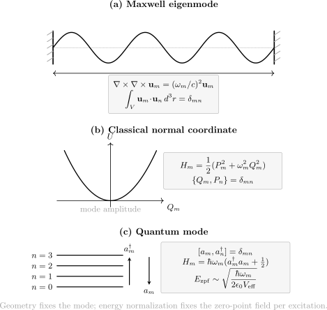
A conservative Maxwell eigenmode supplies one canonical pair $(Q_m,P_m)$. Quantization fixes the equally spaced spectrum and the electric-field scale per excitation. Geometry and normalization are therefore part of the coupling constant, not decorative details.

Canonical Quantization

Promote the normal coordinates to operators with

$$\begin{aligned} [Q_\mu,P_\nu] &= i\hbar\delta_{\mu\nu}, \\ [Q_\mu,Q_\nu] &= 0, \qquad [P_\mu,P_\nu] &= 0. \end{aligned}$$

Define

$$\begin{aligned} a_\mu &= \sqrt{ \frac{\omega_\mu}{2\hbar} } Q_\mu + \frac{i}{ \sqrt{2\hbar\omega_\mu} } P_\mu, \\ a_\mu^\dagger &= \sqrt{ \frac{\omega_\mu}{2\hbar} } Q_\mu - \frac{i}{ \sqrt{2\hbar\omega_\mu} } P_\mu. \end{aligned}$$

Then

$$[a_\mu,a_\nu^\dagger] = \delta_{\mu\nu}, \qquad [a_\mu,a_\nu] = 0,$$

and the inverse relations are

$$\begin{aligned} Q_\mu &= \sqrt{ \frac{\hbar}{2\omega_\mu} } \left( a_\mu+a_\mu^\dagger \right), \\ P_\mu &= -i \sqrt{ \frac{\hbar\omega_\mu}{2} } \left( a_\mu-a_\mu^\dagger \right). \end{aligned}$$

Substitution gives

$$H_{\mathrm{field}} = \sum_\mu \hbar\omega_\mu \left( a_\mu^\dagger a_\mu + \frac12 \right).$$

This is a tensor product of oscillator Hilbert spaces, or equivalently the bosonic Fock space built from the chosen one-mode basis. The general occupation-number construction remains canonical on Fock Space and Mode Occupations.

Constrained field commutator

The canonical momentum density in this source-free Coulomb-gauge problem is

$$\boldsymbol\Pi_{\mathrm T} = \epsilon_0 \dot{\mathbf A}_{\mathrm T} = -\epsilon_0\mathbf E_{\mathrm T}.$$

The equal-time field commutator is transverse:

$$\left[ A_{{\mathrm T},i}(\mathbf r), \Pi_{{\mathrm T},j}(\mathbf r') \right] = i\hbar \delta_{ij}^{\mathrm T} (\mathbf r,\mathbf r').$$

The kernel $\delta^{\mathrm T}$ projects onto the allowed transverse mode space and incorporates the boundary conditions. Replacing it by an unconstrained three-component delta function would reintroduce unphysical longitudinal coordinates.

The field-theory derivation of canonical field brackets is developed on From Phase Space to Canonical Quantization.

Electric and Magnetic Field Operators

For real standing-wave modes, the Schrödinger-picture field operators at a reference time are

$$\begin{aligned} \mathbf A_{\mathrm T}(\mathbf r) ={}& \sum_\mu \sqrt{ \frac{\hbar}{ 2\epsilon_0\omega_\mu } } \, \mathbf u_\mu(\mathbf r) \\ &\quad\times \left( a_\mu+a_\mu^\dagger \right), \\ \mathbf E_{\mathrm T}(\mathbf r) ={}& i \sum_\mu \sqrt{ \frac{\hbar\omega_\mu}{ 2\epsilon_0 } } \, \mathbf u_\mu(\mathbf r) \\ &\quad\times \left( a_\mu-a_\mu^\dagger \right), \\ \mathbf B(\mathbf r) ={}& \sum_\mu \sqrt{ \frac{\hbar}{ 2\epsilon_0\omega_\mu } } \, \nabla\times\mathbf u_\mu(\mathbf r) \\ &\quad\times \left( a_\mu+a_\mu^\dagger \right). \end{aligned}$$

Hermiticity is explicit because the $\mathbf u_\mu$ are real. In the Heisenberg picture,

$$a_\mu(t) = a_\mu(0)e^{-i\omega_\mu t}.$$

It is then useful to split the field into positive- and negative-frequency parts:

$$\mathbf E_{\mathrm T} = \mathbf E^{(+)} + \mathbf E^{(-)}, \qquad \mathbf E^{(-)} = \left( \mathbf E^{(+)} \right)^\dagger.$$

For complex traveling-wave modes,

$$\mathbf E^{(+)}(\mathbf r,t) = i \sum_\mu \sqrt{ \frac{\hbar\omega_\mu}{ 2\epsilon_0 } } \, \mathbf u_\mu(\mathbf r) a_\mu e^{-i\omega_\mu t}.$$

The positive-frequency part contains annihilation operators. This convention is central to absorption photodetection and normally ordered optical correlations.

Unit check

Because $\int|\mathbf u_\mu|^2d^3r=1$, $|\mathbf u_\mu|\sim V^{-1/2}$. The coefficient

$$\sqrt{ \frac{\hbar\omega_\mu}{\epsilon_0} } \mathbf u_\mu$$

has units of electric field. A missing square root of volume or an inconsistent continuum delta function can therefore be detected dimensionally before any rate is calculated.

Plane Waves in a Periodic Box

Take a cubic quantization box of volume $V=L^3$ with periodic boundary conditions. The allowed wave vectors are

$$\mathbf k = \frac{2\pi}{L} \mathbf n, \qquad \mathbf n\in\mathbb Z^3.$$

For each nonzero $\mathbf k$, choose two real orthonormal polarization vectors $\boldsymbol\epsilon_{\mathbf k\lambda}$ satisfying

$$\mathbf k \mathbin{\cdot} \boldsymbol\epsilon_{\mathbf k\lambda} = 0, \qquad \lambda=1,2.$$

A normalized complex mode is

$$\mathbf u_{\mathbf k\lambda}(\mathbf r) = \frac{ \boldsymbol\epsilon_{\mathbf k\lambda} }{ \sqrt V } e^{i\mathbf k\cdot\mathbf r}, \qquad \omega_{\mathbf k} = c|\mathbf k|.$$

The positive-frequency electric field is

$$\begin{aligned} \mathbf E^{(+)}(\mathbf r,t) ={}& i \sum_{\mathbf k,\lambda} \sqrt{ \frac{ \hbar\omega_{\mathbf k} }{ 2\epsilon_0V } } \\ &\times \boldsymbol\epsilon_{\mathbf k\lambda} a_{\mathbf k\lambda} e^{i(\mathbf k\cdot\mathbf r-\omega_{\mathbf k}t)}. \end{aligned}$$

Its Hermitian conjugate supplies $\mathbf E^{(-)}$. The Hamiltonian is

$$H_{\mathrm{field}} = \sum_{\mathbf k,\lambda} \hbar\omega_{\mathbf k} \left( a_{\mathbf k\lambda}^\dagger a_{\mathbf k\lambda} + \frac12 \right).$$

What the box means

The quantization box is usually bookkeeping, not a physical cavity. It:

• discretizes the continuum;
• makes plane waves normalizable;
• assigns a temporary field amplitude proportional to $V^{-1/2}$;
• converts sums into integrals in the infinite-volume limit.

No prediction may depend on this arbitrary $V$. In free-space emission, for example, the squared coupling to one plane-wave mode scales as $1/V$, while the number of available modes in a frequency interval scales as $V$. The factors cancel.

The $\mathbf k=0$ coordinate is not a propagating transverse photon mode with positive frequency and is omitted from this radiation expansion.

Traveling waves and double counting

The labels $\mathbf k$ and $-\mathbf k$ denote distinct traveling directions and have independent annihilation operators. Hermiticity relates the positive- and negative-frequency pieces, not $a_{\mathbf k}$ to $a_{-\mathbf k}^\dagger$.

Confusion arises when formulas for real classical standing-wave coordinates are mixed with formulas for complex traveling-wave operators. Either basis is valid, but the independent degrees of freedom must be counted once.

Continuum Normalization

As $V\to\infty$,

$$\sum_{\mathbf k} \longrightarrow \frac{V}{(2\pi)^3} \int d^3k.$$

Define continuum operators by

$$a_\lambda(\mathbf k) = \sqrt{ \frac{V}{(2\pi)^3} } a_{\mathbf k\lambda}.$$

They satisfy

$$\left[ a_\lambda(\mathbf k), a_{\lambda'}^\dagger(\mathbf k') \right] = \delta_{\lambda\lambda'} \delta^{(3)}(\mathbf k-\mathbf k').$$

The electric field becomes

$$\begin{aligned} \mathbf E^{(+)}(\mathbf r,t) ={}& i \sum_{\lambda=1}^{2} \int \frac{d^3k}{(2\pi)^{3/2}} \sqrt{ \frac{\hbar\omega_{\mathbf k}}{ 2\epsilon_0 } } \\ &\times \boldsymbol\epsilon_{\mathbf k\lambda} a_\lambda(\mathbf k) e^{i(\mathbf k\cdot\mathbf r-\omega_{\mathbf k}t)}. \end{aligned}$$

Continuum annihilation operators carry dimensions inherited from the delta function. They are operator-valued distributions, not ordinary single-oscillator operators.

Normalized wave-packet modes

A physical pulse mode is built from a square-integrable spectral amplitude:

$$A_f^\dagger = \sum_\lambda \int d^3k\, f_\lambda(\mathbf k) a_\lambda^\dagger(\mathbf k),$$

with

$$\sum_\lambda \int d^3k\, |f_\lambda(\mathbf k)|^2 = 1.$$

Then

$$[A_f,A_f^\dagger] = 1.$$

The state $A_f^\dagger|0\rangle$ is a normalizable one-photon wave packet. A monochromatic plane wave in infinite volume is an idealized delta-normalized mode, not a normalizable pulse.

Photon Number

The number operator of mode $\mu$ is

$$N_\mu = a_\mu^\dagger a_\mu.$$

Its eigenstates obey

$$\begin{aligned} N_\mu|n_\mu\rangle &= n_\mu|n_\mu\rangle, \\ a_\mu^\dagger|n_\mu\rangle &= \sqrt{n_\mu+1} |n_\mu+1\rangle, \\ a_\mu|n_\mu\rangle &= \sqrt{n_\mu} |n_\mu-1\rangle. \end{aligned}$$

The energy in that mode is

$$E_{n_\mu} = \hbar\omega_\mu \left( n_\mu+\frac12 \right).$$

Photon Number States develops phase properties, source preparation, counting statistics, and nonclassicality. Here the key point is structural: photon number is an occupation number in a declared mode basis.

Basis dependence

For a passive unitary mode change,

$$c_j = \sum_\mu U_{j\mu}a_\mu, \qquad U^\dagger U=I,$$

the total occupation of the retained mode set is invariant:

$$\sum_j c_j^\dagger c_j = \sum_\mu a_\mu^\dagger a_\mu.$$

Individual occupations are not invariant. A photon in one path superposition can be a photon in a single output mode after a beam splitter.

A transformation mixing $a$ and $a^\dagger$ is different. Time-dependent boundaries, parametric amplification, and changes between inequivalent positive-frequency definitions can produce a Bogoliubov transformation and need not preserve the original photon number.

Vacuum and Zero-Point Fluctuations

The multimode vacuum satisfies

$$a_\mu|0\rangle = 0$$

for every retained mode. For one real mode, define the local electric zero-point amplitude vector

$$\boldsymbol{\mathcal E}_\mu(\mathbf r) = \sqrt{ \frac{\hbar\omega_\mu}{ 2\epsilon_0 } } \mathbf u_\mu(\mathbf r).$$

Its field contribution is

$$\mathbf E_\mu(\mathbf r) = i \boldsymbol{\mathcal E}_\mu(\mathbf r) \left( a_\mu-a_\mu^\dagger \right).$$

The vacuum mean vanishes,

$$\langle0| \mathbf E_\mu(\mathbf r) |0\rangle = 0,$$

but a Cartesian component has nonzero variance:

$$\left\langle0\left| E_{\mu,i}^2(\mathbf r) \right|0\right\rangle = |\mathcal E_{\mu,i}(\mathbf r)|^2.$$

In a number state,

$$\left\langle n\left| E_{\mu,i}^2(\mathbf r) \right|n\right\rangle = (2n+1) |\mathcal E_{\mu,i}(\mathbf r)|^2.$$

The $1$ is the zero-point contribution. It reflects the oscillator commutator and cannot be removed while preserving both field quadratures.

Ordering matters

An ideal absorption detector is governed by a normally ordered quantity such as

$$\langle \mathbf E^{(-)} \mathbin{\cdot} \mathbf E^{(+)} \rangle.$$

For the vacuum this is zero. A symmetrized field variance retains a half-quantum per mode. These facts are compatible because they are different operator orderings tied to different measurement models.

“Vacuum fluctuations” therefore do not mean that an ideal ground-state photodetector continually absorbs real photons from empty space. They mean that field quadratures have irreducible quantum variance and nontrivial commutators. Ordered spectra determine whether a system can absorb from or emit into the field. See Thermal and Vacuum Noise for the open-system frequency-domain dictionary.

Zero-point energy

The free-field vacuum energy is formally

$$E_{\mathrm{vac}} = \frac12 \sum_\mu \hbar\omega_\mu.$$

For an infinite continuum this diverges. The formal sum is not a finite absolute laboratory observable. Measurable boundary-dependent energies, radiative shifts, and forces require a consistent subtraction, regularization, renormalization, or effective-theory matching procedure.

It is equally misleading to say that every phenomenon called a vacuum effect is caused by an independently observable sea of zero-point energy. Vacuum fluctuations, field commutators, radiation reaction, and virtual-process bookkeeping can be redistributed by representation while final observables remain invariant.

Mode Volume and Coupling Strength

For a plane wave in a box,

$$|\mathbf u_{\mathbf k\lambda}|^2 = \frac1V,$$

so the field amplitude per excitation scales as

$$E_{\mathrm{zpf}} \sim \sqrt{ \frac{\hbar\omega}{ 2\epsilon_0V } }.$$

For a standing cavity mode, the field is not spatially uniform. A useful effective mode volume at emitter position $\mathbf r_0$ and dipole direction $\mathbf e_d$ is, for a lossless nondispersive dielectric,

$$V_{\mathrm{eff}} (\mathbf r_0,\mathbf e_d) = \frac{ \displaystyle \int d^3r\, \epsilon_r(\mathbf r) |\mathbf E_c(\mathbf r)|^2 }{ \displaystyle \epsilon_r(\mathbf r_0) | \mathbf e_d \mathbin{\cdot} \mathbf E_c(\mathbf r_0) |^2 }.$$

$\mathbf E_c$ is any consistently normalized classical mode profile; its overall amplitude cancels. Under the assumptions above, the projected zero-point scale can be written schematically as

$$E_{\mathrm{zpf},d}(\mathbf r_0) = \sqrt{ \frac{ \hbar\omega }{ 2\epsilon_0 \epsilon_r(\mathbf r_0) V_{\mathrm{eff}} } }.$$

The corresponding electric-dipole coupling is

$$g = - \frac{ \mathbf d_{eg} \mathbin{\cdot} \mathbf E_{\mathrm{zpf}}(\mathbf r_0) }{ \hbar },$$

up to the phase convention used for the mode and atomic states.

Quantization volume is not effective mode volume

These two volumes answer different questions:

• Quantization volume $V$ is an arbitrary box used to normalize continuum plane waves. It cancels from physical free-space predictions.
• Effective mode volume $V_{\mathrm{eff}}$ characterizes the spatial concentration and polarization overlap of a physical resonator mode. It affects measurable coupling strengths.

Substituting one for the other is a common source of erroneous cavity and spontaneous-emission rates.

When the textbook formula fails

The simple integral above is not universal.

Dispersive media. Electromagnetic energy density involves frequency derivatives of material response, not merely $\epsilon|\mathbf E|^2$. The material degrees of freedom carrying dispersion must be represented consistently.

Absorptive media. A field-only Hermitian normal-mode expansion is generally inadequate. Macroscopic QED introduces reservoir-assisted noise operators tied to the absorptive response and electromagnetic Green tensor.

Open resonators. Outgoing-wave resonances have complex frequencies and spatially divergent quasinormal profiles. Their normalization, mode volume, and completeness require an open-system or scattering formulation; a naive finite integral of $|\mathbf E|^2$ is not valid.

Strongly nonlocal or microscopic media. A local scalar permittivity may itself fail. Mode volume cannot repair an inadequate material model.

Degenerate or multimode systems. A single scalar $V_{\mathrm{eff}}$ can hide polarization, interference, and nonorthogonality. The Green tensor or a validated multimode model is often the safer object.

Worked Example: One-Dimensional Cavity

Consider a cavity of length $L$ and transverse area $A$, with one polarization and perfect mirrors at $x=0$ and $x=L$. A normalized standing-wave mode is

$$\mathbf u_m(\mathbf r) = \mathbf e_y \sqrt{ \frac{2}{AL} } \sin\left( \frac{m\pi x}{L} \right),$$

with

$$\omega_m = \frac{m\pi c}{L}, \qquad m=1,2,\ldots.$$

The normalization follows from

$$\int_0^L \sin^2\left( \frac{m\pi x}{L} \right) dx = \frac L2.$$

At an electric antinode,

$$|\mathbf u_m|_{\max} = \sqrt{ \frac{2}{AL} }.$$

The local zero-point electric amplitude is therefore

$$E_{\mathrm{zpf}}^{\max} = \sqrt{ \frac{\hbar\omega_m}{ \epsilon_0AL } }.$$

The effective mode volume at the antinode is

$$V_{\mathrm{eff}} = \frac{AL}{2},$$

so the same result follows from

$$E_{\mathrm{zpf}}^{\max} = \sqrt{ \frac{\hbar\omega_m}{ 2\epsilon_0V_{\mathrm{eff}} } }.$$

The factor of two is not a contradiction. It records that the standing-wave intensity is concentrated at antinodes rather than uniform throughout the geometric volume $AL$.

Worked Example: Free-Space Mode Density

In a large periodic box, the number of wave vectors in a shell $[k,k+dk]$ is

$$dN_k = 2 \frac{V}{(2\pi)^3} 4\pi k^2dk,$$

where the factor of two counts transverse polarizations. With $\omega=ck$,

$$\rho(\omega) \equiv \frac{dN}{d\omega} = \frac{V\omega^2}{ \pi^2c^3 }.$$

The density per unit volume is

$$\frac{\rho(\omega)}{V} = \frac{\omega^2}{ \pi^2c^3 }.$$

This density of states combines with the $V^{-1/2}$ field amplitude in transition rates. It also supplies the mode counting behind blackbody radiation once each mode is thermally populated.

Boundary geometry, dimensionality, waveguides, cavities, and material dispersion all modify the density of states. Replacing it by the free-space formula in a structured environment defeats the purpose of modeling that environment.

A Normalization Workflow

Before using a quantized field in a calculation:

1. Solve the classical wave problem. State boundaries, material response, gauge, polarization, and whether the spectrum is discrete or continuous.
2. Identify independent modes. Avoid double counting complex-conjugate classical coordinates or polarization labels.
3. Choose one normalization. Record the mode-function inner product and dimensions.
4. Reduce the classical energy. Verify explicitly that each retained coordinate contributes $(P_\mu^2+\omega_\mu^2Q_\mu^2)/2$.
5. Quantize the coordinates. Check $[a_\mu,a_\nu^\dagger]=\delta_{\mu\nu}$ or the declared continuum delta function.
6. Reconstruct the fields. Confirm Hermiticity and Maxwell’s equations.
7. Check energy per excitation. One application of $a_\mu^\dagger$ must raise the energy by $\hbar\omega_\mu$.
8. Check units and volume cancellation. Artificial box factors must cancel from observables.
9. Validate the environment model. Loss, dispersion, leakage, and nonlocal response may require Green-function or reservoir quantization.

This procedure is more reliable than importing a familiar electric-field prefactor from a different geometry.

Common Mistakes

Quantizing a frequency without defining a mode

A frequency does not specify spatial profile, direction, polarization, bandwidth, or boundary conditions. Those data determine the field operator that couples to matter.

Treating all three polarizations as physical

Free radiation has two transverse polarizations per nonzero wave vector. Longitudinal electric fields are constrained by sources rather than being a third photon polarization.

Mixing box and continuum commutators

$\delta_{\mathbf k\mathbf k'}$ and $\delta^{(3)}(\mathbf k-\mathbf k')$ carry different normalization and dimensions. Switching sums to integrals without rescaling operators changes the field amplitude.

Forgetting Hermiticity

$\mathbf E^{(+)}$ is not the full electric field. The observable field is $\mathbf E^{(+)}+\mathbf E^{(-)}$.

Calling the box volume a cavity mode volume

The former is arbitrary continuum bookkeeping; the latter measures physical field concentration and overlap.

Assigning classical random amplitudes to the vacuum

Some Gaussian observables can be represented by stochastic variables, but the vacuum also has operator ordering, commutators, and measurement backaction that an ordinary classical random field does not reproduce universally.

Inferring detector clicks from a symmetrized variance

An ideal absorber samples normally ordered positive- and negative-frequency fields. Nonzero vacuum quadrature variance does not imply a nonzero ideal vacuum count rate.

Dropping zero-point energy inconsistently

A constant can be omitted from isolated finite-mode dynamics, but boundary-dependent energies and matter couplings require a consistent comparison. Neither retaining a divergent bare sum nor deleting every vacuum effect by slogan is a calculation.

Using lossless normalization in an open resonator

Radiating and absorptive modes are not ordinary square-integrable Hermitian normal modes. Complex-frequency resonances need an appropriate open-system normalization and a check of completeness.

Assuming photon number is basis independent

Total occupation is preserved by passive unitary mixing of a fixed mode set, but individual mode occupations depend on basis. Transformations mixing creation and annihilation operators can change even the total number defined by the original basis.

Continue to Field Theory

This page quantizes free transverse radiation modes in a fixed background and uses them in the nonrelativistic AMO setting. Continue through the Bridge to QFT Roadmap for:

• canonical quantization of the free electromagnetic field with constraints;
• covariant gauge fixing and unphysical polarization bookkeeping;
• photon propagators and Green functions;
• charged relativistic matter fields;
• interacting quantum electrodynamics;
• regularization and renormalization;
• the relation between few-mode Hamiltonians and effective field theory.

Harmonic Oscillator to Fields supplies the general oscillator-to-free-field dictionary. The present page specializes that dictionary to electromagnetic modes and laboratory normalization.

Exercises

1. Recover the oscillator Hamiltonian

Starting from

$$\mathbf A_{\mathrm T} = \frac{Q(t)}{\sqrt{\epsilon_0}} \mathbf u(\mathbf r),$$

with

$$\int_V|\mathbf u|^2d^3r=1$$

and

$$\nabla\times\nabla\times\mathbf u = \frac{\omega^2}{c^2}\mathbf u,$$

derive

$$H = \frac12 \left( \dot Q^2+\omega^2Q^2 \right).$$

State the boundary assumption used.

Solution

The fields are

$$\mathbf E_{\mathrm T} = - \frac{\dot Q}{\sqrt{\epsilon_0}} \mathbf u, \qquad \mathbf B = \frac{Q}{\sqrt{\epsilon_0}} \nabla\times\mathbf u.$$

The electric energy is

$$\frac{\epsilon_0}{2} \int_V\mathbf E_{\mathrm T}^2d^3r = \frac{\dot Q^2}{2} \int_V|\mathbf u|^2d^3r = \frac{\dot Q^2}{2}.$$

For the magnetic part, integration by parts gives

$$\begin{aligned} \mathcal I_B \equiv{}& \int_V |\nabla\times\mathbf u|^2d^3r \\ ={}& \mathcal J_B+\mathcal B, \\ \mathcal J_B \equiv{}& \int_V \mathbf u \mathbin{\cdot} \left( \nabla\times\nabla\times\mathbf u \right) d^3r. \end{aligned}$$

The boundary term vanishes when the Maxwell curl–curl operator is self-adjoint under the chosen perfectly reflecting or periodic boundary conditions. Therefore

$$\int_V |\nabla\times\mathbf u|^2d^3r = \frac{\omega^2}{c^2}.$$

Using $1/(\mu_0\epsilon_0)=c^2$,

$$\frac{1}{2\mu_0} \int_V\mathbf B^2d^3r = \frac{\omega^2Q^2}{2}.$$

Adding the two contributions gives the required oscillator Hamiltonian.

2. Check the ladder normalization

Using the definitions of $a$ and $a^\dagger$ on this page, verify $[a,a^\dagger]=1$ and derive $H=\hbar\omega(a^\dagger a+1/2)$.

Solution

Write

$$a = \alpha Q+i\beta P, \qquad a^\dagger = \alpha Q-i\beta P,$$

where

$$\alpha = \sqrt{\frac{\omega}{2\hbar}}, \qquad \beta = \frac{1}{\sqrt{2\hbar\omega}}.$$

Then

$$\begin{aligned} [a,a^\dagger] &= -i\alpha\beta[Q,P] + i\alpha\beta[P,Q] \\ &= 2\alpha\beta\hbar = 1. \end{aligned}$$

The inverse relations give

$$Q = \sqrt{\frac{\hbar}{2\omega}} (a+a^\dagger),$$

and

$$P = -i \sqrt{\frac{\hbar\omega}{2}} (a-a^\dagger).$$

Substitution into $H=(P^2+\omega^2Q^2)/2$, followed by $aa^\dagger=a^\dagger a+1$, yields

$$H = \hbar\omega \left( a^\dagger a+\frac12 \right).$$

3. Field variance in a number state

For one field component,

$$E = i\mathcal E_0 (a-a^\dagger),$$

show that $\langle n|E|n\rangle=0$ and

$$\langle n|E^2|n\rangle = (2n+1)\mathcal E_0^2.$$

Solution

$E$ changes photon number by one, so its diagonal matrix element in a number state vanishes:

$$\langle n|E|n\rangle = 0.$$

Squaring gives

$$E^2 = -\mathcal E_0^2 \left( a^2 -aa^\dagger -a^\dagger a +a^{\dagger2} \right).$$

The $a^2$ and $a^{\dagger2}$ terms have zero diagonal expectation. Using

$$\langle n|aa^\dagger|n\rangle = n+1$$

and

$$\langle n|a^\dagger a|n\rangle = n,$$

one finds

$$\langle n|E^2|n\rangle = (2n+1)\mathcal E_0^2.$$

At $n=0$, the remaining $\mathcal E_0^2$ is the vacuum quadrature variance.

4. Vacuum variance versus absorption

For one mode,

$$E^{(+)} = i\mathcal E_0a, \qquad E^{(-)} = -i\mathcal E_0a^\dagger.$$

Evaluate in the vacuum:

$$\langle E^{(-)}E^{(+)}\rangle$$

and

$$\frac12 \langle E^{(-)}E^{(+)} + E^{(+)}E^{(-)} \rangle.$$

Interpret the difference.

Solution

Normal ordering gives

$$\langle0| E^{(-)}E^{(+)} |0\rangle = \mathcal E_0^2 \langle0|a^\dagger a|0\rangle = 0.$$

For the symmetrized product,

$$\begin{aligned} \mathcal S_E \equiv{}& E^{(-)}E^{(+)} + E^{(+)}E^{(-)}, \\ \mathcal V_E \equiv{}& \frac12 \langle0| \mathcal S_E |0\rangle, \\ \mathcal V_E ={}& \frac{\mathcal E_0^2}{2} \langle0| a^\dagger a+aa^\dagger |0\rangle \\ ={}& \frac{\mathcal E_0^2}{2}. \end{aligned}$$

The numerical factor differs from the full real-quadrature variance because the symmetrized expression here uses the positive- and negative-frequency pieces. The normal-ordered absorption signal vanishes in vacuum, while the symmetrized quadrature noise retains a half-quantum. A detector model selects which ordering is operationally relevant.

5. Box-to-continuum rescaling

Given

$$[a_{\mathbf k\lambda}, a_{\mathbf k'\lambda'}^\dagger] = \delta_{\mathbf k\mathbf k'} \delta_{\lambda\lambda'},$$

show that

$$a_\lambda(\mathbf k) = \sqrt{ \frac{V}{(2\pi)^3} } a_{\mathbf k\lambda}$$

has the continuum commutator stated on this page.

Solution

In the large-box limit, the discrete Kronecker delta corresponds to

$$\delta_{\mathbf k\mathbf k'} \longrightarrow \frac{(2\pi)^3}{V} \delta^{(3)} (\mathbf k-\mathbf k').$$

Therefore

$$\begin{aligned} \left[ a_\lambda(\mathbf k), a_{\lambda'}^\dagger(\mathbf k') \right] ={}& \frac{V}{(2\pi)^3} \delta_{\lambda\lambda'} \delta_{\mathbf k\mathbf k'} \\ \longrightarrow{}& \delta_{\lambda\lambda'} \delta^{(3)} (\mathbf k-\mathbf k'). \end{aligned}$$

This rescaling is also what removes the explicit box volume from the continuum field integral.

6. Derive the free-space density of states

Count electromagnetic modes in a periodic volume $V$ and derive

$$\rho(\omega) = \frac{V\omega^2}{ \pi^2c^3 }.$$

Then explain why a free-space transition rate can be independent of $V$.

Solution

One allowed $\mathbf k$ point occupies volume $(2\pi)^3/V$ in $\mathbf k$ space. The number in a spherical shell is

$$dN = 2 \frac{V}{(2\pi)^3} 4\pi k^2dk,$$

including two transverse polarizations. Since $k=\omega/c$ and $dk=d\omega/c$,

$$dN = \frac{V\omega^2}{ \pi^2c^3 } d\omega.$$

Hence the stated density follows. A dipole coupling to one box-normalized plane wave has $|g_{\mathbf k\lambda}|^2\propto1/V$. Golden-rule rates sum over final modes, contributing $\rho(\omega)\propto V$. The artificial volume cancels.

7. Standing-wave effective volume

For

$$u_m(x) = \sqrt{ \frac{2}{AL} } \sin\left( \frac{m\pi x}{L} \right),$$

compute the effective mode volume at an antinode and show that halving the transverse area increases the zero-point field by $\sqrt2$ at fixed $\omega_m$ and $L$.

Solution

In vacuum,

$$V_{\mathrm{eff}} = \frac{ \int_V|u_m|^2d^3r }{ |u_m|_{\max}^2 }.$$

The numerator is one by normalization, while

$$|u_m|_{\max}^2 = \frac{2}{AL}.$$

Thus

$$V_{\mathrm{eff}} = \frac{AL}{2}.$$

The zero-point field is

$$E_{\mathrm{zpf}}^{\max} = \sqrt{ \frac{\hbar\omega_m}{ 2\epsilon_0V_{\mathrm{eff}} } } = \sqrt{ \frac{\hbar\omega_m}{ \epsilon_0AL } }.$$

Replacing $A$ by $A/2$ multiplies the amplitude by $\sqrt{A/(A/2)}=\sqrt2$.

8. Passive mode mixing

Let

$$c = \frac{a+b}{\sqrt2}, \qquad d = \frac{a-b}{\sqrt2}.$$

Show that $c^\dagger c+d^\dagger d=a^\dagger a+b^\dagger b$. Express $a^\dagger|0\rangle$ in the $c,d$ basis and interpret the result.

Solution

Direct substitution gives

$$\begin{aligned} c^\dagger c+d^\dagger d ={}& \frac12 \left( a^\dagger+b^\dagger \right) \left( a+b \right) \\ &+ \frac12 \left( a^\dagger-b^\dagger \right) \left( a-b \right) \\ ={}& a^\dagger a+b^\dagger b. \end{aligned}$$

Inverting the transformation,

$$a^\dagger = \frac{ c^\dagger+d^\dagger }{ \sqrt2 }.$$

Therefore

$$a^\dagger|0\rangle = \frac{ |1_c,0_d\rangle + |0_c,1_d\rangle }{ \sqrt2 }.$$

The state has one photon in total in either basis, but definite occupation of mode $a$ becomes a superposition of occupations in the $c,d$ basis.

References

• P. A. M. Dirac, “The Quantum Theory of the Emission and Absorption of Radiation,” Proceedings of the Royal Society A 114, 243–265 (1927). Foundational operator treatment of radiation emission and absorption.
• C. Cohen-Tannoudji, J. Dupont-Roc, and G. Grynberg, Photons and Atoms: Introduction to Quantum Electrodynamics, Wiley (1989; online edition 2007). Detailed canonical and multipolar formulations, constraints, and mode quantization.
• L. Mandel and E. Wolf, “Quantization of the Free Electromagnetic Field,” in Optical Coherence and Quantum Optics, Cambridge University Press (1995). Authoritative free-field and optical-coherence conventions.
• G. Grynberg, A. Aspect, and C. Fabre, “Quantization of Free Radiation,” in Introduction to Quantum Optics, Cambridge University Press (2010). Pedagogical derivation from classical normal coordinates to radiation operators.
• R. Loudon, The Quantum Theory of Light, 3rd ed., Oxford University Press (2000). Standard treatment of field quantization, photon states, and light–matter processes.
• P. W. Milonni, The Quantum Vacuum: An Introduction to Quantum Electrodynamics, Academic Press (1994). Zero-point fluctuations, operator ordering, radiative effects, and vacuum-energy cautions.
• S. Scheel and S. Y. Buhmann, “Macroscopic QED: Concepts and Applications,” Acta Physica Slovaca 58, 675–809 (2008). Quantization in dispersive and absorbing media using reservoir fields and Green tensors.
• C. Sauvan, J. P. Hugonin, I. S. Maksymov, and P. Lalanne, “Theory of the Spontaneous Optical Emission of Nanosize Photonic and Plasmon Resonators,” Physical Review Letters 110, 237401 (2013). Open, lossy, dispersive quasinormal-mode normalization and generalized mode-volume cautions.
• E. S. C. Ching, P. T. Leung, A. Maassen van den Brink, W. M. Suen, S. S. Tong, and K. Young, “Quasinormal-Mode Expansion for Waves in Open Systems,” Reviews of Modern Physics 70, 1545–1554 (1998). Mathematical structure, completeness, and limitations of open-system resonant modes.