Input–Output Theory Overview

Input–output theory connects a localized optical degree of freedom to the traveling fields that enter and leave its ports. For a cavity, it answers three questions in one framework:

1. How does an incident field drive the intracavity mode?
2. How does coupling to external modes damp that intracavity excitation?
3. What reflected, transmitted, or emitted field reaches a detector?

The central distinction is between a dimensionless intracavity annihilation operator $\hat a$ and a traveling-field operator $\hat b_{\rm in}(t)$ or $\hat b_{\rm out}(t)$, whose squared amplitude is a photon flux. A cavity may contain one photon on average while emitting much less than one photon in a short time bin; conversely, a bright reflected beam can result from interference between the incident field and a weak field radiated by the cavity.

For one Markovian port, the laboratory dictionary is

$$\begin{gathered} \text{intracavity damping} \quad\longleftrightarrow\quad \kappa, \\ \text{incident drive} \quad\longleftrightarrow\quad \hat b_{\rm in}(t), \\ \text{detected field} \quad\longleftrightarrow\quad \hat b_{\rm out}(t), \\ \hat b_{\rm out} = \hat b_{\rm in} + \sqrt\kappa\,\hat a. \end{gathered}$$

The final plus sign is a phase convention. This page consistently pairs it with a minus input term in the cavity Langevin equation. Other references use $\hat b_{\rm out}=\hat b_{\rm in}-\sqrt\kappa\,\hat a$ and a corresponding opposite drive phase. Reflection phases change under this relabeling; observable powers and consistently computed interference do not.

Canonical Scope

This page is the practical cavity-optics overview. It owns

• the distinction between an internal resonance and external traveling continua;
• energy-decay, amplitude-decay, lifetime, linewidth, and quality-factor conventions;
• the input–output boundary condition at one or several cavity ports;
• coherent intracavity build-up;
• empty-cavity reflection and transmission amplitudes;
• undercoupling, overcoupling, impedance matching, and internal loss;
• ringdown, output flux, and the fields supplied to optical detectors;
• an experimental workflow for fitting cavity response without mixing incompatible conventions.

Input–Output Theory in the open-systems volume owns the general Markov derivation, quantum stochastic boundary condition, arbitrary coupling operator $L$, and continuous-measurement connection. Quantum Langevin Equations owns the general Heisenberg-picture noise calculus.

The present page specializes that machinery to the empty optical cavity and its ports. Cavity QED uses the resulting susceptibility but adds an emitter, cooperativity, polariton poles, Purcell channeling, and cavity-enhanced readout. The Jaynes–Cummings Model adds the exact closed-system spectrum and excitation-exchange dynamics. Later pages Nonlinear Quantum Optics derives nonlinear optical response and parametric gain; the present input–output boundary condition then connects such intracavity dynamics to measured traveling fields.

Conventions at a Glance

The following conventions are used throughout:

• $\omega_c$ is the bare cavity angular frequency.
• A coherent probe has angular frequency $\omega_d$.
• The drive detuning is $\Delta=\omega_d-\omega_c$.
• $\kappa_j$ is the energy-decay rate through port $j$.
• $\kappa_{\rm int}$ is the total unmonitored internal-loss rate.
• $\kappa=\sum_j\kappa_j+\kappa_{\rm int}$ is the total energy-decay rate.
• The intracavity field amplitude decays at rate $\kappa/2$.
• Traveling fields obey $[\hat b_j(t),\hat b_k^\dagger(t')]=\delta_{jk}\delta(t-t')$.
• $|\beta_{\rm in}|^2$ is an incident photon flux, not an intracavity photon number.

All rates and linewidths are angular frequencies unless explicitly divided by $2\pi$.

The Internal Cavity Mode

An ideal closed cavity has discrete electromagnetic normal modes. Restricting attention to one resonance gives

$$\hat H_c = \hbar\omega_c \left( \hat a^\dagger\hat a+\frac12 \right), \qquad [\hat a,\hat a^\dagger]=1.$$

The occupation

$$\hat n_c=\hat a^\dagger\hat a$$

is dimensionless. Its expectation is the mean number of excitations stored in that selected cavity mode.

A real cavity is open. A partially transmitting mirror, waveguide coupler, or radiation aperture turns the closed-cavity normal mode into a resonance with a finite linewidth. Input–output theory represents it as a localized quasimode $\hat a$ coupled to one or more continua. This is accurate when one isolated resonance dominates and the external coupling varies slowly across its linewidth.

Quantized Electromagnetic Modes owns the conservative normal-mode quantization and field normalization. The present page begins where radiation leakage makes a closed normal-mode description insufficient.

Stored energy and photon number

Ignoring the zero-point offset, the stored cavity energy is

$$E_c = \hbar\omega_c \langle\hat n_c\rangle.$$

For a coherent cavity state $|\alpha\rangle$,

$$\langle\hat a\rangle=\alpha, \qquad \langle\hat n_c\rangle=|\alpha|^2.$$

The complex amplitude $\alpha$ has no units in this normalization. It should not be compared directly with $\beta_{\rm in}$, which has units $\mathrm{s}^{-1/2}$.

External Continua

Each open port supports traveling modes over a continuum of frequencies. Let $\hat b_j(\omega)$ annihilate a continuum excitation in port $j$, with

$$[ \hat b_j(\omega), \hat b_k^\dagger(\omega') ] = \delta_{jk}\delta(\omega-\omega').$$

Factors of $2\pi$ sometimes appear on the right-hand side and then move into the Fourier transform. A consistent temporal normalization is

$$\hat b_{j,\rm in}(t) = \frac{1}{\sqrt{2\pi}} \int d\omega\, e^{-i(\omega-\omega_d)t} \hat b_{j,\rm in}(\omega),$$

which gives

$$[ \hat b_{j,\rm in}(t), \hat b_{k,\rm in}^\dagger(t') ] = \delta_{jk}\delta(t-t').$$

The corresponding normally ordered photon flux is

$$\Phi_{j,\rm in}(t) = \left\langle \hat b_{j,\rm in}^\dagger(t) \hat b_{j,\rm in}(t) \right\rangle.$$

Thus $\hat b(t)$ has units $\mathrm{s}^{-1/2}$. A normalized incoming wave-packet mode

$$\hat B_f = \int dt\, f^*(t)\hat b_{\rm in}(t).$$

The mode is normalized by

$$\int dt\,|f(t)|^2=1,$$

is dimensionless and obeys $[\hat B_f,\hat B_f^\dagger]=1$. This distinction between a flux field and an integrated wave-packet mode prevents many dimensional mistakes.

Vacuum is still an input field

An undriven port is not deleted from the equations. It carries vacuum input with

$$\begin{aligned} \langle \hat b_{\rm in}^\dagger(t) \hat b_{\rm in}(t') \rangle_{\rm vac} &=0, \\ \langle \hat b_{\rm in}(t) \hat b_{\rm in}^\dagger(t') \rangle_{\rm vac} &=\delta(t-t'). \end{aligned}$$

The first line says the normally ordered incident photon flux vanishes. The second preserves field commutators and supplies the fluctuations associated with damping. Replacing an unused port by the number zero while retaining its loss rate is not a valid quantum model.

Coupling a Mode to a Continuum

In a rotating-wave and narrowband description, one port can be represented by a coupling Hamiltonian of the form

$$\begin{aligned} \hat H_{\rm int} ={}& i\hbar \int d\omega\, \sqrt{ \frac{\kappa(\omega)}{2\pi} } \\ &\times \left[ \hat b^\dagger(\omega)\hat a - \hat a^\dagger\hat b(\omega) \right]. \end{aligned}$$

The phase of $\hat b$ has been chosen to match this page’s input–output sign convention. The important physics is the coupling magnitude and its frequency dependence.

Formally solving the continuum equations and substituting them into the cavity equation produces

• a frequency shift from the principal-value part of the reservoir response;
• a memory kernel from the finite reservoir correlation time;
• a fluctuating incident-field operator.

The cavity frequency $\omega_c$ below is understood to include the relevant renormalized shift. The Markov approximation replaces the coupling by its value near resonance,

$$\kappa(\omega)\simeq\kappa(\omega_c),$$

and extends the narrow frequency integral so the memory kernel becomes local in time.

This requires

• a coupling density that is nearly flat across the cavity linewidth;
• a reservoir correlation time short compared with cavity dynamics;
• no resolved propagation delay or coherent return path;
• a rotating-wave description adequate near the selected resonance;
• ports that can be treated as independent input channels.

Photonic band edges, narrow external resonances, long feedback loops, frequency-dependent mirror response, and overlapping quasimodes can violate these assumptions.

Damping Rate and Linewidth

Suppose the cavity couples to ports with rates $\kappa_j$ and to unmonitored internal-loss channels with total rate $\kappa_{\rm int}$. The total rate is

$$\kappa = \sum_j\kappa_j + \kappa_{\rm int}.$$

With vacuum inputs and no internal Hamiltonian beyond the cavity resonance,

$$\langle\hat a(t)\rangle = e^{-\kappa t/2} \langle\hat a(0)\rangle,$$

whereas

$$\langle\hat n_c(t)\rangle = e^{-\kappa t} \langle\hat n_c(0)\rangle.$$

Therefore

• the field-amplitude decay rate is $\kappa/2$;
• the energy-decay rate is $\kappa$;
• the photon or energy lifetime is $\tau_E=1/\kappa$;
• the field-amplitude lifetime is $\tau_A=2/\kappa$.

The empty-cavity intensity response is Lorentzian. Its full width at half maximum is

$$\delta\omega_{\rm FWHM}=\kappa.$$

In ordinary frequency,

$$\delta\nu_{\rm FWHM} = \frac{\kappa}{2\pi}.$$

The loaded quality factor is

$$Q_{\rm loaded} = \frac{\omega_c}{\kappa}.$$

Some communities define $\kappa$ as the field-amplitude decay rate or quote a half width rather than a full width. A fitted number is incomplete unless the definition is stated.

Cavity Langevin Equation

Move to a frame rotating at the drive frequency $\omega_d$, with $\Delta=\omega_d-\omega_c$. For a linear cavity,

$$\begin{aligned} \dot{\hat a} ={}& \left( i\Delta-\frac{\kappa}{2} \right)\hat a \\ &- \sum_j \sqrt{\kappa_j}\, \hat b_{j,\rm in}(t) - \sqrt{\kappa_{\rm int}}\, \hat\xi_{\rm int}(t). \end{aligned}$$

The operator $\hat\xi_{\rm int}$ collects internal-loss noise. If internal loss contains physically distinct reservoirs, each should have its own rate and input operator.

Dropping every input operator would give damped deterministic motion, but it would also make the canonical commutator decay:

$$[ \hat a(t), \hat a^\dagger(t) ] \stackrel{\rm no\ noise}{=} e^{-\kappa t}.$$

The vacuum inputs restore the missing part and keep $[\hat a(t),\hat a^\dagger(t)]=1$. Dissipation and quantum noise are two aspects of the same port coupling.

Input and Output Fields

For each monitored Markovian port,

$$\hat b_{j,\rm out}(t) = \hat b_{j,\rm in}(t) + \sqrt{\kappa_j}\,\hat a(t).$$

The output is a coherent sum of a prompt incident field and the field radiated by the cavity. Reflection minima and phase flips arise from interference between these amplitudes. They cannot be obtained by adding incident and emitted intensities.

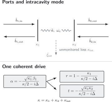
A localized mode $\hat a$ couples to two monitored ports and one unmonitored loss bath. Driving port 1 produces intracavity amplitude $\alpha$, reflection $r$, and transmission $t$ in the sign and detuning convention used on this page.

What the boundary condition means

The relation is local at the coupling plane. It does not include propagation phases between the coupler and a remote detector. Those phases should be added to the transfer path, not hidden in $\kappa_j$.

The input field is defined before interaction with the cavity; the output field is defined after interaction. Quantum causality determines which input–system correlations vanish at equal-time limits and is handled carefully in the full stochastic derivation. The compact boundary condition should not be manipulated as though every operator at time $t$ were an independent commuting number.

Internal loss is another port

Absorption, scattering into uncollected modes, and imperfect confinement can be modeled as additional bath ports. Their outputs exist physically even if no detector monitors them. Treating internal loss as a rate without its noise input is acceptable for mean classical amplitudes but incomplete for quantum fluctuations, commutators, and output states.

Coherent Drive and Intracavity Build-Up

Drive port 1 with a coherent amplitude plus zero-mean fluctuations:

$$\hat b_{1,\rm in}(t) = \beta_1+\delta\hat b_{1,\rm in}(t).$$

The incident photon flux is

$$\Phi_{\rm in}=|\beta_1|^2.$$

Let $\alpha=\langle\hat a\rangle$ and take every other input to have zero mean. Then

$$\dot\alpha = \left( i\Delta-\frac{\kappa}{2} \right)\alpha - \sqrt{\kappa_1}\,\beta_1.$$

The steady-state amplitude is

$$\alpha_{\rm ss} = - \frac{ \sqrt{\kappa_1}\,\beta_1 }{ \kappa/2-i\Delta }.$$

Define the cavity susceptibility

$$\chi_c(\Delta) = \frac{1}{\kappa/2-i\Delta}.$$

Then

$$\alpha_{\rm ss} = -\sqrt{\kappa_1}\, \chi_c(\Delta)\beta_1.$$

The mean intracavity photon number is

$$\bar n_c = \frac{ \kappa_1|\beta_1|^2 }{ (\kappa/2)^2+\Delta^2 }.$$

This Lorentzian build-up is largest on resonance. It scales with the coupling rate through the driven port but is limited by the total linewidth, including every monitored and unmonitored decay channel.

Reflection and Transmission

Assume port 1 is coherently driven, while port 2 and the internal-loss ports have zero mean input. The output means are

$$\begin{aligned} \beta_{1,\rm out} &= \beta_1+\sqrt{\kappa_1}\,\alpha_{\rm ss}, \\ \beta_{2,\rm out} &= \sqrt{\kappa_2}\,\alpha_{\rm ss}. \end{aligned}$$

Define complex amplitude coefficients relative to the incident field:

$$r(\Delta) = \frac{\beta_{1,\rm out}}{\beta_1}, \qquad t(\Delta) = \frac{\beta_{2,\rm out}}{\beta_1}.$$

Substituting the steady-state cavity amplitude gives

$$r(\Delta) = 1 - \frac{ \kappa_1 }{ \kappa/2-i\Delta },$$

and

$$t(\Delta) = - \frac{ \sqrt{\kappa_1\kappa_2} }{ \kappa/2-i\Delta }.$$

The direct term $1$ in $r$ is the prompt reflected input in this port convention. The second term is radiation from the cavity. A deep reflection dip is destructive interference between them, not evidence that the cavity emits no field.

Lossless single-sided cavity

For one external port and no internal loss,

$$\kappa=\kappa_1, \qquad \kappa_2=\kappa_{\rm int}=0.$$

The reflection coefficient becomes

$$r(\Delta) = \frac{ -\kappa/2-i\Delta }{ \kappa/2-i\Delta }.$$

Its magnitude is unity at every frequency:

$$|r(\Delta)|=1.$$

The cavity cannot absorb or transmit energy, so it acts as a frequency-dependent phase shifter. On resonance $r(0)=-1$ in this convention. Far from resonance, $r\rightarrow1$.

Measuring only reflected power would miss this lossless cavity completely: $R=|r|^2=1$ everywhere. Phase-sensitive detection or interferometric reference reveals the resonance.

Two-sided cavity and internal loss

For drive through port 1, define

$$\mathcal D(\Delta) = \left(\frac{\kappa}{2}\right)^2+\Delta^2.$$

The reflected and transmitted power fractions are

$$R(\Delta) = \frac{ \left[ (\kappa_2+\kappa_{\rm int}-\kappa_1)/2 \right]^2 + \Delta^2 }{ \mathcal D(\Delta) },$$

and

$$T(\Delta) = \frac{ \kappa_1\kappa_2 }{ \mathcal D(\Delta) }.$$

The fraction leaving through internal-loss channels is

$$A(\Delta) = \frac{ \kappa_1\kappa_{\rm int} }{ \mathcal D(\Delta) }.$$

For passive vacuum loss,

$$R(\Delta)+T(\Delta)+A(\Delta)=1.$$

This identity is a strong convention and algebra check. If a passive empty-cavity model predicts a sum larger than one, a sign, linewidth, or normalization has been mixed incorrectly.

On resonance,

$$r(0) = \frac{ \kappa_2+\kappa_{\rm int}-\kappa_1 }{ \kappa },$$

and

$$t(0) = - \frac{ 2\sqrt{\kappa_1\kappa_2} }{ \kappa }.$$

A symmetric lossless two-sided cavity has $\kappa_1=\kappa_2=\kappa/2$. It gives $r(0)=0$ and $t(0)=-1$: all resonant power exits port 2, with a convention-dependent phase.

Critical coupling and impedance matching

For a one-sided cavity with external coupling $\kappa_{\rm ext}$ and internal loss $\kappa_{\rm int}$,

$$r(0) = \frac{ \kappa_{\rm int}-\kappa_{\rm ext} }{ \kappa_{\rm int}+\kappa_{\rm ext} }.$$

Three regimes follow:

• undercoupled: $\kappa_{\rm ext}<\kappa_{\rm int}$;
• critically coupled: $\kappa_{\rm ext}=\kappa_{\rm int}$;
• overcoupled: $\kappa_{\rm ext}>\kappa_{\rm int}$.

At critical coupling, $r(0)=0$. All resonant incident power enters the cavity and leaves through internal-loss channels in this one-port model. The zero reflection results from destructive interference, while the energy disposition is fixed by the available decay channels.

For a two-sided cavity driven through port 1, zero resonant reflection instead requires

$$\kappa_1=\kappa_2+\kappa_{\rm int}.$$

Calling both situations “critical coupling” is common, but the transmitted and absorbed fractions differ. The port topology must accompany the phrase.

Coupling efficiencies

The escape probability for a cavity excitation through port $j$ is

$$\eta_j^{\rm esc} = \frac{\kappa_j}{\kappa}.$$

The total monitored escape efficiency is

$$\eta_{\rm mon}^{\rm esc} = \frac{ \sum_{j\in{\rm monitored}}\kappa_j }{ \kappa }.$$

Escape efficiency is not the same as propagation transmission, spatial mode matching, or detector quantum efficiency. Those later losses multiply the probability that an escaped excitation produces the intended record.

Frequency-Domain Scattering Matrix

For several linear ports, the empty-cavity amplitude scattering matrix has the compact form

$$S_{jk}(\omega) = \delta_{jk} - \frac{ \sqrt{\kappa_j\kappa_k} }{ \kappa/2-i(\omega-\omega_c) }.$$

The diagonal term contains the prompt path. The rank-one resonant term comes from entering and leaving through the cavity mode.

If every loss bath is included as an explicit port, the full passive scattering matrix is unitary on the real-frequency axis. The submatrix restricted to experimentally monitored ports is generally not unitary when internal loss is traced out. Apparent nonunitarity is then missing information and energy in unobserved channels, not a violation of quantum mechanics.

The simple matrix assumes no nonresonant background except the identity prompt path. Real devices can have cable delay, mirror propagation phase, mode mismatch, Fano interference, or a direct bypass channel. Those effects should be modeled explicitly rather than absorbed into a complex, frequency-dependent “$\kappa$.”

Time-Domain Response and Ringdown

For a stable linear cavity, the intracavity field is a causal convolution of the past input with the impulse response:

$$\begin{aligned} \hat a(t) ={}& - \sum_j\sqrt{\kappa_j} \\ &\times \int_{-\infty}^{t}ds\, e^{(i\Delta-\kappa/2)(t-s)} \hat b_{j,\rm in}(s) \\ &- \sqrt{\kappa_{\rm int}} \\ &\times \int_{-\infty}^{t}ds\, e^{(i\Delta-\kappa/2)(t-s)} \hat\xi_{\rm int}(s). \end{aligned}$$

A drive varying slowly compared with $1/\kappa$ approximately follows the instantaneous steady state. A pulse with bandwidth comparable to or larger than $\kappa$ excites transient dynamics and is reshaped by the cavity.

Cavity ringdown

Prepare amplitude $\alpha_0$ and turn the coherent drive off at $t=0$. Then

$$\alpha(t) = \alpha_0 e^{(i\Delta-\kappa/2)t},$$

and

$$\bar n_c(t) = |\alpha_0|^2e^{-\kappa t}.$$

With vacuum incident fields, the emitted photon flux through port $j$ is

$$\Phi_{j,\rm out}(t) = \kappa_j\bar n_c(t).$$

Integrating the entire ringdown gives

$$N_j = \int_0^\infty dt\, \Phi_{j,\rm out}(t) = \frac{\kappa_j}{\kappa} |\alpha_0|^2.$$

The initial photons divide among channels according to their rates. Summing over every external and internal port returns $|\alpha_0|^2$.

Ringdown directly measures the energy-decay rate when the detector response is faster than the decay and no slow mode, thermal repopulation, or coherent feedback distorts the exponential. A field-amplitude measurement decays with time constant $2/\kappa$; direct intensity decays with time constant $1/\kappa$.

What a Detector Sees

Detectors act on traveling output fields, not directly on $\hat a$. Input–output theory supplies the operator entering each measurement model.

Output photon flux

At port $j$,

$$\Phi_{j,\rm out}(t) = \left\langle \hat b_{j,\rm out}^\dagger(t) \hat b_{j,\rm out}(t) \right\rangle.$$

Using the boundary relation,

$$\begin{aligned} \Phi_{j,\rm out} ={}& \langle \hat b_{j,\rm in}^\dagger \hat b_{j,\rm in} \rangle + \kappa_j \langle\hat a^\dagger\hat a\rangle \\ &+ \sqrt{\kappa_j} \langle \hat b_{j,\rm in}^\dagger\hat a + \hat a^\dagger\hat b_{j,\rm in} \rangle. \end{aligned}$$

The final line is interference. For vacuum input and spontaneous cavity emission, the emitted flux is $\kappa_j\langle\hat n_c\rangle$. For a coherently driven reflection experiment, omitting the interference terms destroys the reflection dip and gives the wrong energy balance.

Photon Counting owns the detector POVM, efficiency, dark counts, dead time, timing response, and number-resolution limits.

Output quadratures

Balanced homodyne detection measures a mode of $\hat b_{j,\rm out}(t)$ selected by the local oscillator. The prompt coherent input is often subtracted electronically or displaced optically, leaving fluctuations radiated by the cavity. The subtraction changes the recorded mean, not the underlying output-field commutator.

Homodyne and Heterodyne Detection owns local-oscillator mode selection, quadrature calibration, heterodyne added vacuum, and optical tomography. The trajectory pages own conditional state updates driven by the resulting record.

Spectra and correlations

Output spectra and correlation functions follow by replacing each output operator with its input–output expression and evaluating the required multi-time averages. An empty linear cavity filters Gaussian inputs linearly. An atom, nonlinear medium, or parametric interaction inside the cavity can imprint non-Gaussian correlations, squeezing, or antibunching on the output.

The boundary condition alone does not compute internal multi-time correlators. Those come from the cavity’s Hamiltonian and open-system dynamics, often through the quantum regression theorem or a stochastic trajectory calculation.

Relation to Open Systems

The same physical port appears in several equivalent descriptions. For cavity port $j$, define

$$\hat L_j = \sqrt{\kappa_j}\,\hat a.$$

Then the port contributes

$$\mathcal D[\hat L_j]\rho = \kappa_j\mathcal D[\hat a]\rho$$

to the unconditional master equation, where

$$\mathcal D[\hat a]\rho = \hat a\rho\hat a^\dagger - \frac12 \left\{ \hat a^\dagger\hat a,\rho \right\}.$$

For vacuum inputs and a linear cavity in the drive frame,

$$\begin{aligned} \dot\rho ={}& - \frac{i}{\hbar} [ \hat H_{\rm rot}+\hat H_{\rm drive}, \rho ] \\ &+ \sum_j \kappa_j\mathcal D[\hat a]\rho + \kappa_{\rm int}\mathcal D[\hat a]\rho. \end{aligned}$$

The Hamiltonian terms are

$$\hat H_{\rm rot} = -\hbar\Delta\, \hat a^\dagger\hat a,$$

and, for drive through port 1,

$$\hat H_{\rm drive} = i\hbar\sqrt{\kappa_1} \left( \beta_1^*\hat a - \beta_1\hat a^\dagger \right).$$

They reproduce the mean Langevin equation used above.

The dictionary is

• master equation: discard all output records and retain $\mathcal D[L_j]\rho$;
• Langevin equation: retain the incident quantum fields as operator noise;
• input–output relation: retain the outgoing fields;
• quantum trajectory: condition the state on a specified measurement of one or more outgoing fields.

Combining all vacuum loss terms into $\kappa\mathcal D[a]\rho$ is sufficient for unconditional cavity dynamics. It is insufficient for predicting which port carries an emitted photon or how efficiently that output is monitored. Port-resolved operators must be retained for those questions.

Coherent input versus a classical force

Moving a coherent input amplitude into $\hat H_{\rm drive}$ is a displacement of the bath description. Vacuum fluctuations remain in the input channel. Replacing the whole quantum input by a deterministic force gives the correct mean for a linear cavity but loses shot noise and cannot predict output quantum statistics.

Thermal, Squeezed, and Nonclassical Inputs

The boundary condition does not require vacuum input. For a stationary thermal Markov field with occupation $\bar n$,

$$\begin{aligned} \langle \hat b_{\rm in}^\dagger(t) \hat b_{\rm in}(t') \rangle &= \bar n\,\delta(t-t'), \\ \langle \hat b_{\rm in}(t) \hat b_{\rm in}^\dagger(t') \rangle &= (\bar n+1)\delta(t-t'). \end{aligned}$$

A squeezed input also has anomalous correlations such as $\langle\hat b_{\rm in}(t)\hat b_{\rm in}(t')\rangle$. A finite-bandwidth squeezed source is generally not perfectly delta correlated and may require an explicit auxiliary mode or colored-noise model.

For nonclassical wave packets containing one or a few photons, the input state is not summarized by a coherent amplitude. One can retain temporal input modes explicitly, use Fock-state master equations, or solve a scattering problem. The empty-cavity transfer amplitude remains useful, but a classical mean-field calculation does not determine the output state.

When the Simple Cavity Model Fails

The one-mode Markov model should be enlarged when

• several cavity resonances overlap within a linewidth;
• external coupling varies appreciably across the signal bandwidth;
• a nearby waveguide band edge or narrow resonance creates memory;
• propagation delay and coherent feedback are dynamically resolved;
• mirror dispersion or absorption cannot be represented by a flat loss bath;
• the cavity couples ultrastrongly enough that rotating-wave port coupling becomes questionable;
• nonlinear dynamics makes a single linear susceptibility inadequate;
• the output contains spatial or polarization modes not represented by the declared ports.

A useful repair is often to promote the structured part of the environment to an explicit system mode. The remaining broad continuum can then be treated Markovian at the enlarged boundary.

Fitting a Cavity Responsibly

1. Declare the topology. State which ports are driven, monitored, or treated as internal loss.
2. Fix signs and detuning. Record whether $\Delta=\omega_d-\omega_c$ or the opposite and whether the output boundary has a plus or minus radiated term.
3. Calibrate the off-resonant baseline. Include propagation phase, insertion loss, mode mismatch, and any direct bypass path.
4. Measure complex response when possible. Power alone cannot reveal a lossless one-sided resonance and may not distinguish undercoupling from overcoupling.
5. Cross-check linewidth in time and frequency. The intensity FWHM $\kappa$ and ringdown lifetime $1/\kappa$ should agree after instrument response is included.
6. Separate total and partial rates. Linewidth gives $\kappa$; reflection depth, transmission, calibrated loss, or independent ringdown channels are needed to infer $\kappa_j$ and $\kappa_{\rm int}$.
7. Propagate calibration uncertainty. Coupling fractions near critical coupling can be highly sensitive to small baseline and mode-matching errors.
8. Test passivity and residuals. Verify power conservation for the fitted model and inspect systematic deviations that signal Fano backgrounds, extra modes, or frequency-dependent coupling.

Common Mistakes

Equating the cavity mode with the output beam

$\hat a$ is dimensionless and localized; $\hat b_{\rm out}(t)$ is a flux field. Their units, commutators, and physical locations differ.

Confusing energy and amplitude decay rates

Energy and photon number decay at $\kappa$; field amplitude decays at $\kappa/2$. The intensity-response FWHM is $\kappa$ in this convention.

Deleting vacuum inputs

An unused lossy port still supplies vacuum fluctuations. Dropping its noise operator makes commutators decay and generally corrupts output noise.

Mixing boundary signs

Taking the Langevin equation from one convention and the output relation from another changes interference and can violate power conservation.

Adding intensities instead of amplitudes

Reflection contains a prompt input and cavity radiation. Their cross term is the resonance.

Treating every linewidth as intrinsic loss

The loaded linewidth contains all escape and internal-loss rates. A broad resonance can be deliberately overcoupled and still have little absorption.

Inferring coupling regime from power without a baseline model

Mode mismatch, etalons, cable delay, and direct paths can change a reflection dip. Complex response and ringdown provide stronger constraints.

Applying a steady-state formula to a broadband pulse

A pulse with bandwidth comparable to $\kappa$ is filtered and rings down. Its output cannot be found by evaluating $r$ or $t$ only at the carrier.

Combining ports too early

The total dissipator may depend only on $\kappa$, but port-resolved transmission, collection efficiency, and measurement records depend on each $\kappa_j$.

Exercises

Exercise 1: Flux fields and wave-packet modes

Let

$$[ \hat b(t), \hat b^\dagger(t') ] = \delta(t-t')$$

and define

$$\hat B_f = \int dt\,f^*(t)\hat b(t).$$

Determine the units of $\hat b(t)$ and $f(t)$. Show that $[\hat B_f,\hat B_f^\dagger]=1$ when $\int dt\,|f(t)|^2=1$.

Solution

The delta function has units of inverse time, so $\hat b(t)$ has units $\mathrm{s}^{-1/2}$. For $\hat B_f$ to be dimensionless, $f(t)$ must also have units $\mathrm{s}^{-1/2}$.

Using the field commutator,

$$\begin{aligned} [ \hat B_f,\hat B_f^\dagger ] ={}& \int dt\,dt'\, f^*(t)f(t') \\ &\times [ \hat b(t),\hat b^\dagger(t') ]. \end{aligned}$$

Substitution gives

$$\begin{aligned} [ \hat B_f,\hat B_f^\dagger ] &= \int dt\,dt'\, f^*(t)f(t') \delta(t-t') \\ &= \int dt\,|f(t)|^2 = 1. \end{aligned}$$

Thus a normalized temporal wave packet is one ordinary dimensionless bosonic mode, while $\hat b(t)$ is a continuum flux field.

Exercise 2: Vacuum noise preserves the cavity commutator

For one resonant port, consider

$$\dot{\hat a} = -\frac{\kappa}{2}\hat a - \sqrt\kappa\,\hat b_{\rm in}(t).$$

Assume $[\hat a(0),\hat a^\dagger(0)]=1$, the initial cavity and input commute, and the input has the white-noise commutator. Solve formally and show that $[\hat a(t),\hat a^\dagger(t)]=1$.

Solution

The formal solution is

$$\begin{aligned} \hat a(t) ={}& e^{-\kappa t/2}\hat a(0) \\ &- \sqrt\kappa \int_0^t ds\, e^{-\kappa(t-s)/2} \hat b_{\rm in}(s). \end{aligned}$$

Initial system–field cross commutators vanish. Therefore

$$\begin{aligned} [ \hat a(t),\hat a^\dagger(t) ] ={}& e^{-\kappa t} \\ &+ \kappa \int_0^t ds\, e^{-\kappa(t-s)}. \end{aligned}$$

The integral is

$$\kappa \int_0^t ds\, e^{-\kappa(t-s)} = 1-e^{-\kappa t}.$$

Hence

$$[ \hat a(t),\hat a^\dagger(t) ] = e^{-\kappa t} + 1-e^{-\kappa t} = 1.$$

Without the input-noise term, only the first contribution would remain and the canonical algebra would decay.

Exercise 3: Intracavity response and linewidth

A cavity is driven through port 1 with photon flux $\Phi_{\rm in}=|\beta_1|^2$. Starting from

$$\dot\alpha = \left( i\Delta-\frac{\kappa}{2} \right)\alpha - \sqrt{\kappa_1}\beta_1,$$

find the steady-state photon number. Show that its intensity full width at half maximum is $\kappa$.

Solution

Setting $\dot\alpha=0$ gives

$$\alpha_{\rm ss} = - \frac{ \sqrt{\kappa_1}\beta_1 }{ \kappa/2-i\Delta }.$$

Therefore

$$\bar n_c(\Delta) = \frac{ \kappa_1\Phi_{\rm in} }{ (\kappa/2)^2+\Delta^2 }.$$

On resonance,

$$\bar n_c(0) = \frac{ 4\kappa_1\Phi_{\rm in} }{ \kappa^2 }.$$

Half maximum occurs when

$$\left(\frac{\kappa}{2}\right)^2+\Delta^2 = 2\left(\frac{\kappa}{2}\right)^2,$$

so

$$|\Delta|=\frac{\kappa}{2}.$$

The two half-maximum points are separated by $\kappa$, so the intensity FWHM is $\kappa$ in angular-frequency units.

Exercise 4: A lossless one-port cavity can be invisible in power

For

$$r(\Delta) = \frac{ -\kappa/2-i\Delta }{ \kappa/2-i\Delta },$$

show that reflected power is independent of detuning. What observable still reveals the cavity?

Solution

The squared magnitudes of numerator and denominator are equal:

$$\left| -\frac{\kappa}{2}-i\Delta \right|^2 = \left| \frac{\kappa}{2}-i\Delta \right|^2 = \frac{\kappa^2}{4}+\Delta^2.$$

Therefore

$$R(\Delta)=|r(\Delta)|^2=1.$$

The cavity changes the phase of $r$. In this convention it changes from the far-detuned value $r\simeq1$ to $r(0)=-1$ on resonance. Interferometry, homodyne detection, or network analysis of the complex reflected amplitude reveals that phase response even though a power-only scan is flat.

Exercise 5: Power conservation for a two-sided cavity

Using

$$\mathcal D = \left(\frac{\kappa}{2}\right)^2+\Delta^2$$

and $\kappa=\kappa_1+\kappa_2+\kappa_{\rm int}$, verify that the fractions

$$\begin{aligned} R &= \frac{ [(\kappa_2+\kappa_{\rm int}-\kappa_1)/2]^2 + \Delta^2 }{ \mathcal D }, \\ T &= \frac{\kappa_1\kappa_2}{\mathcal D}, \\ A &= \frac{\kappa_1\kappa_{\rm int}}{\mathcal D} \end{aligned}$$

satisfy $R+T+A=1$.

Solution

The numerator of the sum is

$$\begin{aligned} \mathcal N ={}& \frac14 ( \kappa_2+\kappa_{\rm int}-\kappa_1 )^2 + \Delta^2 \\ &+ \kappa_1\kappa_2 + \kappa_1\kappa_{\rm int}. \end{aligned}$$

Let $x=\kappa_2+\kappa_{\rm int}$. Then

$$\begin{aligned} \frac14(x-\kappa_1)^2+\kappa_1x &= \frac14(x+\kappa_1)^2 \\ &= \frac{\kappa^2}{4}. \end{aligned}$$

Thus

$$\mathcal N = \frac{\kappa^2}{4}+\Delta^2 = \mathcal D,$$

and $R+T+A=1$.

Exercise 6: Coupling regime from a resonant reflection

A one-port cavity has

$$\frac{\kappa_{\rm ext}}{2\pi} = 4.0\ \mathrm{MHz}, \qquad \frac{\kappa_{\rm int}}{2\pi} = 1.0\ \mathrm{MHz}.$$

Find its loaded intensity linewidth, resonant reflection amplitude, reflected power, and internally lost power fraction. Classify the coupling regime.

Solution

The loaded rate is the sum:

$$\frac{\kappa}{2\pi} = 5.0\ \mathrm{MHz}.$$

This is the intensity FWHM in ordinary-frequency units. On resonance,

$$\begin{aligned} r(0) &= \frac{ \kappa_{\rm int}-\kappa_{\rm ext} }{ \kappa_{\rm int}+\kappa_{\rm ext} } \\ &= \frac{1-4}{1+4} = -0.6. \end{aligned}$$

Therefore

$$R(0)=|r(0)|^2=0.36.$$

There is no transmission port, so passivity gives

$$A(0)=1-R(0)=0.64.$$

Because $\kappa_{\rm ext}>\kappa_{\rm int}$, the cavity is overcoupled. The negative reflection amplitude encodes the resonant phase flip; power alone would not distinguish its sign.

Exercise 7: Ringdown branching ratios

A cavity initially contains $\bar n_c(0)=10$ photons. Its decay rates are in the ratio

$$\kappa_1:\kappa_2:\kappa_{\rm int} = 5:3:2.$$

The loaded linewidth is $\kappa/(2\pi)=10\ \mathrm{MHz}$. Find the energy lifetime, field-amplitude lifetime, and mean number of photons eventually leaving through each channel.

Solution

The total angular decay rate is

$$\kappa = 2\pi \left( 10\ \mathrm{MHz} \right).$$

The energy lifetime is

$$\tau_E = \frac1\kappa \simeq 15.9\ \mathrm{ns},$$

and the field-amplitude lifetime is

$$\tau_A = \frac2\kappa \simeq 31.8\ \mathrm{ns}.$$

The normalized branching fractions are $0.5$, $0.3$, and $0.2$. Therefore

$$N_1=5, \qquad N_2=3, \qquad N_{\rm int}=2.$$

Their sum equals the initial mean occupation. The internal share is physically emitted into or absorbed by unmonitored bath degrees of freedom even though it does not appear in a collected optical record.

Exercise 8: Same master equation, different collection

Compare two empty cavities with the same total rate $\kappa$. Cavity A has one monitored port with $\kappa_1=\kappa$. Cavity B has $\kappa_1=\kappa/4$ and $\kappa_{\rm int}=3\kappa/4$. Both baths are vacuum.

1. Show that their unconditional undriven master equations are identical.
2. If each starts in $|1\rangle$, find the probability that the photon exits through the monitored port.
3. Explain why the total master equation alone cannot answer the second question.

Solution

For cavity A, the dissipative term is

$$\kappa\mathcal D[\hat a]\rho.$$

For cavity B, the monitored and internal terms add:

$$\begin{aligned} \frac{\kappa}{4} \mathcal D[\hat a]\rho + \frac{3\kappa}{4} \mathcal D[\hat a]\rho &= \kappa\mathcal D[\hat a]\rho. \end{aligned}$$

Thus both have the same unconditional decay of every intracavity observable.

The probability for one initial excitation to leave through port 1 is its branching ratio:

$$P_1=\frac{\kappa_1}{\kappa}.$$

Therefore

$$P_1^{(A)}=1, \qquad P_1^{(B)}=\frac14.$$

Combining channels into one total dissipator erases their physical labels. The port-resolved coupling operators $L_1=\sqrt{\kappa_1}\,a$ and $L_{\rm int}=\sqrt{\kappa_{\rm int}}\,a$ must be retained to predict collection probabilities or measurement records.

References

1. C. W. Gardiner and M. J. Collett, “Input and output in damped quantum systems: Quantum stochastic differential equations and the master equation,” Physical Review A 31, 3761–3774 (1985).
2. M. J. Collett and C. W. Gardiner, “Squeezing of intracavity and traveling-wave light fields produced in parametric amplification,” Physical Review A 30, 1386–1391 (1984).
3. C. W. Gardiner, A. S. Parkins, and M. J. Collett, “Input and output in damped quantum systems. II. Methods in non-white-noise situations and application to inhibition of atomic phase decays,” Journal of the Optical Society of America B 4, 1683–1699 (1987).
4. B. Yurke and J. S. Denker, “Quantum network theory,” Physical Review A 29, 1419–1437 (1984).
5. H. A. Haus, Waves and Fields in Optoelectronics (Prentice-Hall, 1984).
6. H. J. Carmichael, An Open Systems Approach to Quantum Optics, Lecture Notes in Physics m18 (Springer, 1993).
7. C. W. Gardiner and P. Zoller, Quantum Noise, 3rd ed. (Springer, 2004).
8. D. F. Walls and G. J. Milburn, Quantum Optics, 2nd ed. (Springer, 2008).
9. H. M. Wiseman and G. J. Milburn, Quantum Measurement and Control (Cambridge University Press, 2010).
10. A. A. Clerk, M. H. Devoret, S. M. Girvin, F. Marquardt, and R. J. Schoelkopf, “Introduction to quantum noise, measurement, and amplification,” Reviews of Modern Physics 82, 1155–1208 (2010).
11. S. Fan, Ş. E. Kocabaş, and J.-T. Shen, “Input-output formalism for few-photon transport in one-dimensional nanophotonic waveguides,” Physical Review A 82, 063821 (2010).
12. J. Gough and M. R. James, “The series product and its application to quantum feedforward and feedback networks,” IEEE Transactions on Automatic Control 54, 2530–2544 (2009).
13. M. Aspelmeyer, T. J. Kippenberg, and F. Marquardt, “Cavity optomechanics,” Reviews of Modern Physics 86, 1391–1452 (2014).
14. P. Lodahl, S. Mahmoodian, and S. Stobbe, “Interfacing single photons and single quantum dots with photonic nanostructures,” Reviews of Modern Physics 87, 347–400 (2015).
15. F. Lei, J. M. Ward, P. Romagnoli, and S. Nic Chormaic, “Polarization-controlled cavity input–output relations,” Physical Review Letters 124, 103902 (2020).