Photon Antibunching

Photon antibunching is the suppression of nearby photoevents relative to events separated by a longer delay. For a stationary field, the direct temporal criterion is

$$g^{(2)}(\tau) > g^{(2)}(0)$$

for at least one delay $\tau$. A widely used equal-time signature is

$$g^{(2)}(0)<1.$$

Both occur for ideal resonance fluorescence from one two-level emitter, but they answer different questions. The first compares two delays and violates a stationary classical correlation bound. The second compares the equal-time factorial moment with a Poisson reference and is a sufficient optical nonclassicality witness. Outside stationary single-mode settings, antibunching and sub-Poissonian counting statistics need not imply one another.

The physical mechanism is especially transparent for one emitter. Detection of a fluorescence photon leaves a two-level emitter in its ground state. It must be excited again before it can emit another photon, so the conditional emission rate starts at zero and recovers over the excitation and decay timescales.

A defensible antibunching claim identifies the detected mode, source operating point, delay or pulse convention, accidental baseline, timing response, background model, detector artifacts, fit model, and uncertainty. A dip in an unnormalized histogram is not yet such a claim.

Canonical Scope

This page is the canonical home for:

• temporal photon antibunching and its stationary classical inequality;
• the equal-time condition $g^{(2)}(0)<1$ and its relation to sub-Poissonian photon statistics;
• the single-emitter reset mechanism and its jump-operator formulation;
• two-level-emitter antibunching under incoherent and coherent driving;
• continuous-wave and pulsed experimental signatures;
• source-specific effects from background, multiple emitters, timing response, re-excitation, shelving, blinking, and spectral filtering;
• responsible interpretation of antibunching as a nonclassicality and single-emitter diagnostic.

Correlation Functions owns the general definitions of $G^{(2)}$, $g^{(2)}$, normal ordering, coherence hierarchies, and classical correlation bounds. Hanbury Brown–Twiss Interferometry owns the two-channel apparatus, coincidence-histogram construction, accidental normalization, and intensity-interferometry geometry. Photon Counting owns detector POVMs, efficiency calibration, dark counts, dead time, afterpulsing, timing jitter, and response matrices.

Photon Number States owns number-state preparation, one-photon wave packets, source brightness, indistinguishability, and the broader specification of a single-photon source. This page uses those concepts only to interpret antibunching. Identical-particle exchange antibunching belongs to Quantum Statistics Overview.

What the Correlation Measures

Stationary normalized correlation

For one stationary detected field, write

$$\begin{aligned} G^{(2)}(\tau) ={}& \left\langle \hat E^{(-)}(t) \hat E^{(-)}(t+\tau) \right. \\ &\left. \qquad {}\times \hat E^{(+)}(t+\tau) \hat E^{(+)}(t) \right\rangle , \end{aligned}$$

and

$$g^{(2)}(\tau) = \frac{ G^{(2)}(\tau) }{ \left\langle \hat E^{(-)}\hat E^{(+)} \right\rangle^2 }.$$

Normal ordering makes the numerator a joint absorption probability density in the broadband direct-detection model. Stationarity removes the arbitrary origin $t$, but it does not remove the signed delay $\tau$, detector labels, polarization, spectral filter, spatial mode, or timing response.

For a sufficiently ideal stationary counting channel,

$$g^{(2)}(\tau) = \frac{ R(\tau\mid 0) }{ R_{\mathrm{ss}} },$$

where $R(\tau\mid0)$ is the conditional event rate at delay $\tau$ after an event at zero and $R_{\mathrm{ss}}$ is the unconditional steady rate. Thus:

• $g^{(2)}(\tau)>1$ means an event raises the conditional rate at that delay;
• $g^{(2)}(\tau)=1$ means the rate has returned to its uncorrelated baseline;
• $g^{(2)}(\tau)<1$ means an event suppresses the conditional rate.

The word “simultaneous” always refers to an idealized limit or a declared gate. A real instrument reports a time-averaged and response-convolved quantity.

Three statements that should not be collapsed

Temporal antibunching means that the correlation rises away from zero:

$$g^{(2)}(\tau)>g^{(2)}(0)$$

for some $\tau$ in a stationary measurement. This is a comparison between delays.

Equal-time sub-Poissonian behavior means

$$g^{(2)}(0)<1$$

for the specified mode or sufficiently short counting gate. This is a comparison with the Poisson factorial moment.

Ideal single-photon exclusion means

$$g^{(2)}(0)=0.$$

It says that the retained field has no equal-time two-photon contribution under the model. It does not by itself state the source brightness, vacuum probability, mode purity, indistinguishability, or delivery efficiency.

In common continuous-wave fluorescence experiments all three statements may hold. Treating them as definitions of one another hides the assumptions that make them coincide.

Why Antibunching Is Nonclassical

Stationary classical delay bound

Let $I(t)\ge0$ be a stationary classical random intensity. The Cauchy–Schwarz inequality gives

$$\begin{aligned} \left| \mathbb E[ I(t)I(t+\tau) ] \right|^2 \le{}& \mathbb E[I(t)^2] \\ &\times \mathbb E[I(t+\tau)^2] . \end{aligned}$$

Stationarity makes the two second moments equal, so

$$\mathbb E[ I(t)I(t+\tau) ] \le \mathbb E[ I(t)^2 ].$$

After division by $\mathbb E[I]^2$,

$$g_{\mathrm{cl}}^{(2)}(\tau) \le g_{\mathrm{cl}}^{(2)}(0).$$

A calibrated stationary correlation that rises away from zero violates this classical random-intensity bound. The conclusion depends on stationarity and on excluding detector recovery or other artificial short-delay suppression.

This criterion does not require $g^{(2)}(0)<1$. In principle, a curve can rise from $1.2$ at zero to $1.3$ at a later delay and still violate the stationary classical inequality.

Nonnegative Glauber–Sudarshan P bound

An optically classical single-mode state has a nonnegative Glauber–Sudarshan representation,

$$\rho = \int d^2\alpha\, P(\alpha) |\alpha\rangle\langle\alpha|, \qquad P(\alpha)\ge0.$$

For normally ordered equal-time moments, set

$$I_\alpha=|\alpha|^2.$$

Then

$$\begin{aligned} g^{(2)}(0) &= \frac{ \mathbb E_P[I_\alpha^2] }{ \mathbb E_P[I_\alpha]^2 } \\ &= 1+ \frac{ \operatorname{Var}_P(I_\alpha) }{ \mathbb E_P[I_\alpha]^2 } \ge1. \end{aligned}$$

Consequently,

$$g^{(2)}(0)<1$$

is sufficient to rule out every ordinary nonnegative $P$ representation, assuming the measured normally ordered moment and calibration model are valid. It is not a necessary condition for nonclassicality: squeezed vacuum, entangled light, and many other nonclassical states can have $g^{(2)}(0)\ge1$.

Discrete clicks are not enough

Photodetectors produce discrete electronic outcomes even under weak coherent illumination. Attenuated coherent light remains Poissonian,

$$g^{(2)}(0)=1,$$

at every nonzero amplitude in the ideal model. The nonclassical evidence is the calibrated correlation inequality, not the visual fact that a detector clicks.

Relation to Photon Statistics

Factorial moments

For one mode with number operator $\hat n=\hat a^\dagger\hat a$,

$$g^{(2)}(0) = \frac{ \langle \hat n(\hat n-1) \rangle }{ \langle\hat n\rangle^2 }.$$

Since

$$\langle \hat n(\hat n-1) \rangle = \operatorname{Var}(\hat n) + \langle\hat n\rangle^2 - \langle\hat n\rangle,$$

one obtains

$$g^{(2)}(0) = 1+ \frac{ \operatorname{Var}(\hat n) - \langle\hat n\rangle }{ \langle\hat n\rangle^2 }.$$

The Fano factor

$$F := \frac{ \operatorname{Var}(\hat n) }{ \langle\hat n\rangle }$$

therefore satisfies

$$F = 1+ \langle\hat n\rangle \left[ g^{(2)}(0)-1 \right].$$

For this fixed mode or gate, $g^{(2)}(0)<1$ is equivalent to $F<1$. Temporal antibunching of a nonstationary or broadly gated record is not generally equivalent to sub-Poissonian statistics in a different gate.

The Mandel parameter is

$$Q := \frac{ \operatorname{Var}(\hat n)-\langle\hat n\rangle }{ \langle\hat n\rangle } = \langle\hat n\rangle \left[ g^{(2)}(0)-1 \right].$$

Thus $Q<0$ is the same equal-time sub-Poissonian condition under these definitions.

Number states

For a number state $|n\rangle$ with $n\ge1$,

$$g_{|n\rangle}^{(2)}(0) = \frac{ n(n-1) }{ n^2 } = 1-\frac1n.$$

In particular,

$$g_{|1\rangle}^{(2)}(0)=0.$$

The value for $|2\rangle$ is $1/2$, even though the state contains exactly two photons. This is one reason a threshold such as $g^{(2)}(0)<1/2$ must be interpreted within a source model rather than promoted to a universal definition of “one photon.”

Pulsed trials

For a pulsed source, let $N_k$ be the photon number in the declared output mode on trigger $k$. The per-pulse factorial moment is

$$g_{\mathrm p}^{(2)}[0] := \frac{ \langle N_k(N_k-1)\rangle }{ \langle N_k\rangle^2 }.$$

If only zero-, one-, and two-photon sectors are appreciable,

$$\begin{aligned} \bar N &= p_1+2p_2, \\ g_{\mathrm p}^{(2)}[0] &= \frac{ 2p_2 }{ \bar N^2 }. \end{aligned}$$

A measured $g_{\mathrm p}^{(2)}[0]$ does not determine $p_2$ unless $\bar N$ or equivalent brightness information is also known. A source that emits one photon once per million triggers and vacuum otherwise has $g_{\mathrm p}^{(2)}[0]=0$, but it is not a bright on-demand source.

Independent loss

Under mode-independent Bernoulli loss of efficiency $\eta$,

$$\begin{aligned} \langle N_{\mathrm{det}}\rangle &= \eta\langle N\rangle, \\ \langle N_{\mathrm{det}}(N_{\mathrm{det}}-1) \rangle &= \eta^2 \langle N(N-1)\rangle. \end{aligned}$$

The normalized $g^{(2)}$ is therefore unchanged by ideal independent loss. Loss lowers the event rate and enlarges statistical uncertainty. It can also lower the signal fraction relative to fixed background, which fills an observed dip.

Why One Emitter Antibunches

Nilpotent lowering operator

For a two-level emitter,

$$\hat\sigma_- = |g\rangle\langle e|, \qquad \hat\sigma_-^2=0.$$

Let the monitored radiative channel have jump operator

$$\hat L = \sqrt{\Gamma}\, \hat\sigma_-.$$

The equal-time coincidence numerator contains two successive lowering operations:

$$\begin{aligned} G^{(2)}(0) &\propto \operatorname{Tr} \left[ \hat L^\dagger \hat L^\dagger \hat L \hat L \rho_{\mathrm{ss}} \right] \\ &= 0. \end{aligned}$$

Whenever the steady emission rate is nonzero,

$$g^{(2)}(0)=0.$$

This operator identity is the ideal zero-delay exclusion. It is stronger and cleaner than saying that photons “repel” one another. The emitter cannot support two simultaneous excitations in the modeled transition.

State reset after a click

The normalized state immediately after a detected jump is

$$\rho_{\mathrm c}(0^+) = \frac{ \hat L\rho_{\mathrm{ss}}\hat L^\dagger }{ \operatorname{Tr} \left[ \hat L^\dagger\hat L\rho_{\mathrm{ss}} \right] }.$$

For one ideal two-level transition,

$$\rho_{\mathrm c}(0^+) = |g\rangle\langle g|.$$

The next emission requires the drive to rebuild excited-state population. This waiting process, not a force between emitted photons, creates the short-delay deficit.

Jump-superoperator expression

Define

$$\mathcal J\rho := \hat L\rho\hat L^\dagger$$

and let $\mathcal L$ be the unconditional Markovian Liouvillian. The steady count rate is

$$R_{\mathrm{ss}} = \operatorname{Tr} \left[ \mathcal J\rho_{\mathrm{ss}} \right].$$

For $\tau\ge0$, the quantum regression or conditional-jump expression is

$$g^{(2)}(\tau) = \frac{ \operatorname{Tr} \left[ \mathcal J e^{\mathcal L\tau} \left( \mathcal J\rho_{\mathrm{ss}} \right) \right] }{ R_{\mathrm{ss}}^2 }.$$

The inner jump prepares the conditional state, $e^{\mathcal L\tau}$ evolves it, and the outer jump asks for the emission rate at delay $\tau$. This formula is the natural bridge to Quantum Jump Trajectories. It assumes the same Markovian dynamics used to define $\mathcal L$; memory, frequency filtering, or delayed feedback may require an enlarged model.

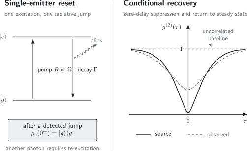
A fluorescence click resets an ideal two-level emitter to $|g\rangle$, so a second click must wait for re-excitation. The solid curve sketches the source correlation; the dashed curve illustrates how finite timing response and background can make the observed dip broader and shallower. Neither curve is a substitute for a declared forward model.

Two-Level Correlation Models

Incoherent excitation

Consider incoherent pumping at rate $R$ and radiative decay at rate $\Gamma$:

$$\dot\rho = R\, \mathcal D[\hat\sigma_+]\rho + \Gamma\, \mathcal D[\hat\sigma_-]\rho,$$

where

$$\mathcal D[\hat c]\rho := \hat c\rho\hat c^\dagger - \frac12 \left\{ \hat c^\dagger\hat c,\rho \right\}.$$

Immediately after an emission, the conditional excited-state probability $p_e(\tau)$ obeys

$$\frac{d p_e}{d\tau} = R(1-p_e) - \Gamma p_e, \qquad p_e(0)=0.$$

The steady population and conditional solution are

$$\begin{aligned} p_e^{\mathrm{ss}} &= \frac{R}{R+\Gamma}, \\ p_e(\tau) &= p_e^{\mathrm{ss}} \left[ 1-e^{-(R+\Gamma)\tau} \right]. \end{aligned}$$

Since the fluorescence rate is $\Gamma p_e$,

$$g^{(2)}(\tau) = 1- e^{-(R+\Gamma)|\tau|}.$$

This model gives a monotonic recovery. The dip narrows as the pump rate increases because re-excitation becomes faster. At very high rates, detector timing response and additional levels often become as important as this two-rate prediction.

Coherent resonant drive

For resonant coherent driving with Rabi frequency $\Omega$,

$$\dot\rho = -i \left[ \frac{\Omega}{2} \left( \hat\sigma_+ + \hat\sigma_- \right), \rho \right] + \Gamma \mathcal D[\hat\sigma_-]\rho.$$

With no additional pure dephasing, the steady resonance-fluorescence result can be written

$$\begin{aligned} g^{(2)}(\tau) &= 1 - e^{-3\Gamma|\tau|/4} f(\tau), \\ f(\tau) &= \cos(\nu|\tau|) + \frac{ 3\Gamma }{ 4\nu } \sin(\nu|\tau|) . \end{aligned}$$

where

$$\nu = \sqrt{ \Omega^2-\frac{\Gamma^2}{16} }.$$

If $\nu$ is imaginary, the trigonometric functions are understood by analytic continuation to hyperbolic functions. At strong drive the correlation shows damped Rabi oscillations: after a photon resets the emitter, the coherent drive cycles population between $|g\rangle$ and $|e\rangle$ before damping returns the system to steady state.

The exact line shape changes with detuning, pure dephasing, polarization selection, coherent laser leakage, and which fluorescence component is filtered. The reliable procedure is to propagate the post-click state with the same calibrated master equation used for the steady state. Optical Bloch Equations owns the one-time driven-state dynamics.

Shelving and blinking

A metastable dark state adds a slow conditional timescale. A common phenomenological form is

$$\begin{aligned} g^{(2)}(\tau) ={}& 1 - (1+a) e^{-|\tau|/\tau_{\mathrm a}} \\ &+ a e^{-|\tau|/\tau_{\mathrm b}}, \qquad \tau_{\mathrm b}\gg\tau_{\mathrm a}, \end{aligned}$$

with $a>0$. The fast term produces antibunching and the slow term produces a bunching shoulder. At zero delay the ideal expression still gives $g^{(2)}(0)=0$.

An antibunching dip and bunching at longer delay are therefore compatible. The dip diagnoses short-time excitation exclusion; the shoulder diagnoses slow switching among emissive and dark configurations. Assigning every feature to a single “lifetime” discards this information.

More than literal two-level atoms

The same conditional-exclusion logic appears in atoms, trapped ions, molecules, color centers, semiconductor quantum dots, and engineered superconducting emitters. Multilevel structure modifies the recovery. Photon blockade and other nonlinear resonators can also suppress two-photon occupation without being literal two-level material systems. The observable remains a correlation of a declared output channel.

Experimental Signatures

Two-channel measurement

The standard laboratory measurement routes one selected source field to two detectors and builds a cross-correlation of their event records. The splitter does not create the source antibunching. Under independent linear loss, it routes the source’s factorial moment into a measurable cross-coincidence.

Using two detectors is important because a single detector’s dead time creates an automatic short-delay exclusion in its autocorrelation. A cross-channel measurement avoids that particular artifact, but it does not eliminate:

• optical leakage between channels;
• electrical cross-talk or shared threshold logic;
• common timing or trigger artifacts;
• detector afterpulsing;
• source-independent correlated background;
• saturation and live-time bias.

The apparatus, lag-histogram estimator, accidental baseline, and uncertainty are developed on Hanbury Brown–Twiss Interferometry. The present question is what a normalized dip says about the source.

Continuous-wave records

For stationary continuous excitation, an ideal narrow lag bin centered at $\tau_k$ has expected coincidence count

$$\mathbb E[C_k] \simeq R_1R_2 T_{\mathrm{acq}} \Delta\tau\, g_{12}^{(2)}(\tau_k),$$

away from record-edge corrections. Here $R_j$ are live-time-corrected channel rates, $T_{\mathrm{acq}}$ is common exposure, and $\Delta\tau$ is the bin width.

The uncorrelated baseline is not necessarily the average of whichever bins look flat. It must account for:

• acquisition gaps and unequal live time;
• rate drift and intermittency;
• start–stop or all-pairs counting conventions;
• lag-dependent exposure near record edges;
• periodic triggers or modulation;
• excluded regions and fit uncertainty.

A continuous-wave antibunching fit commonly returns a correlation timescale, raw dip depth, background-corrected depth, and perhaps a slow blinking timescale. These parameters should not be called lifetimes unless the fitted physical model justifies that identification.

Pulsed records

With repetition period $T_{\mathrm r}$, a delay histogram forms peaks near

$$\tau=mT_{\mathrm r}, \qquad m\in\mathbb Z.$$

Let $A_m$ be a peak area integrated over a declared coincidence window. Under stable independent trials and equal lag exposure,

$$\widehat g_{\mathrm p}^{(2)}[0] \simeq \frac{ A_0 }{ \langle A_m\rangle_{m\ne0} }.$$

This ratio is only a starting estimator. Side peaks are not an unbiased baseline when blinking correlates neighboring pulses, the trigger train has gaps, detector dead time spans several periods, or the source drifts. One may instead fit the complete sequence of peak areas with a trial-to-trial correlation model.

The central area probes two detections associated with one trigger. It should not be replaced by the height of one histogram bin, which depends strongly on timing jitter and arbitrary bin alignment.

Re-excitation within a pulse

An emitter can radiate once, be re-excited before the pump pulse ends, and radiate again. A source may therefore have a single occupied transition and still produce a nonzero same-pulse multiphoton probability.

Suppressing re-excitation can require:

• a pump pulse short compared with the radiative cycle;
• coherent pulse-area control;
• resonant rather than above-band excitation;
• temporal filtering, with its stated efficiency cost;
• a level scheme that prevents immediate return to the pump resonance.

A small continuous-wave zero-delay dip and a small pulsed central-peak area are related diagnostics, not interchangeable numbers.

Measurement Forward Model

Independent background

Let channel $j$ have mean signal rate $S_j$, independent Poisson background $B_j$, and signal fraction

$$\rho_j := \frac{ S_j }{ S_j+B_j }.$$

If the two backgrounds are mutually independent and independent of the signal, then

$$g_{\mathrm{raw}}^{(2)}(\tau)-1 = \rho_1\rho_2 \left[ g_{\mathrm s}^{(2)}(\tau)-1 \right].$$

For symmetric channels with $\rho_1=\rho_2=\rho$,

$$g_{\mathrm{raw}}^{(2)}(\tau) = 1- \rho^2 \left[ 1-g_{\mathrm s}^{(2)}(\tau) \right].$$

Background pulls every dip and peak toward one. For an ideal source with $g_{\mathrm s}^{(2)}(0)=0$,

$$g_{\mathrm{raw}}^{(2)}(0) = 1-\rho_1\rho_2.$$

The correction is invalid for correlated background, leakage of the pump into both channels, source-dependent fluorescence background, or a background estimate taken under a different operating condition.

Worked background example

Suppose both detector channels have signal fraction $0.90$, and the measured raw value is

$$g_{\mathrm{raw}}^{(2)}(0)=0.433.$$

Under the independent-background model,

$$\begin{aligned} g_{\mathrm s}^{(2)}(0) &= 1+ \frac{ g_{\mathrm{raw}}^{(2)}(0)-1 }{ (0.90)^2 } \\ &= 0.30. \end{aligned}$$

The inferred source value is meaningful only with uncertainties on the raw correlation and both signal fractions. It remains an inference, not another raw datum.

Timing response

Let $K(\tau)$ be the normalized relative-time response of the detector pair, including both detector jitters and any synchronization uncertainty:

$$\int d\tau\,K(\tau)=1.$$

For a stationary linear timing model,

$$\begin{aligned} g_{\mathrm{timed}}^{(2)}(\tau)-1 ={}& \int d\tau'\, K(\tau-\tau') \\ &\times \left[ g_{\mathrm{raw}}^{(2)}(\tau')-1 \right]. \end{aligned}$$

Histogram binning performs another average. For a bin of width $\Delta\tau$,

$$\overline g_k^{(2)} = \frac1{\Delta\tau} \int_{\tau_k-\Delta\tau/2}^{\tau_k+\Delta\tau/2} d\tau\, g_{\mathrm{timed}}^{(2)}(\tau).$$

Finite timing resolution conserves the integrated correlation excess or deficit in this ideal convolution model but spreads it over delay. A narrow perfect source dip can therefore appear shallow or unresolved. Deconvolution without regularization and uncertainty propagation can manufacture an overconfident zero.

Multiple independent emitters

Suppose independent emitters contribute mean detected signal rates $s_i$ to the same channel. If their individual equal-time correlations are $g_i^{(2)}(0)$, then

$$\begin{aligned} g_{\mathrm{tot}}^{(2)}(0)-1 = \frac{ \displaystyle \sum_i s_i^2 \left[ g_i^{(2)}(0)-1 \right] }{ \displaystyle \left( \sum_i s_i \right)^2 }. \end{aligned}$$

For ideal antibunched emitters, $g_i^{(2)}(0)=0$, so

$$g_{\mathrm{tot}}^{(2)}(0) = 1- \frac{ \sum_i s_i^2 }{ \left( \sum_i s_i \right)^2 }.$$

Define the effective contributor number

$$N_{\mathrm{eff}} := \frac{ \left( \sum_i s_i \right)^2 }{ \sum_i s_i^2 }.$$

Then

$$g_{\mathrm{tot}}^{(2)}(0) = 1- \frac1{N_{\mathrm{eff}}}.$$

For $N$ equal-brightness emitters, $N_{\mathrm{eff}}=N$ and

$$g_{\mathrm{tot}}^{(2)}(0) = 1-\frac1N.$$

Unequal brightness matters. Two ideal emitters with rates in the ratio $3:1$ give

$$g_{\mathrm{tot}}^{(2)}(0) = 1- \frac{3^2+1^2}{(3+1)^2} = \frac38.$$

This is below $1/2$ even though two emitters are present. The correlation shows that one contributor dominates; by itself it does not count physical objects.

Detector artifacts

Detector behavior can create either sign of correlation:

• dead time and recovery suppress short-delay events and can imitate an antibunching dip in a same-detector record;
• afterpulsing creates a delayed excess, often on a detector-specific timescale;
• electrical or optical cross-talk creates near-zero cross-channel excess;
• saturation changes the live time and makes accidental normalization rate dependent;
• gating can impose a periodic envelope unrelated to source dynamics;
• time-tagger rollover or clock pickup can create narrow repeated structures.

Blocked-input, dark-record, split coherent-light, rate-scaling, channel-swap, and large-time-shift controls are often more informative than adding another free parameter to the source fit.

Spectral and polarization filtering

The detected field is the source field after mode selection. Filtering is not always a passive cosmetic step:

• rejecting uncorrelated background can deepen the measured dip;
• admitting several independent transitions can fill it;
• polarization selection can isolate or mix decay channels;
• a narrow spectral filter has a long impulse response and changes temporal correlations;
• coherent pump leakage can interfere with the emitted field;
• selecting one sideband of resonance fluorescence measures a different correlation from collecting the total fluorescence.

Every quoted $g^{(2)}$ therefore belongs to a stated detection channel, not to an emitter independent of its optical measurement.

Interpreting a Single-Photon Claim

What a value below one establishes

After detector artifacts and calibration uncertainty are controlled,

$$g^{(2)}(0)<1$$

is a sufficient nonclassicality witness for the measured normally ordered field. It also shows a sub-Poissonian factorial moment in the same mode or gate.

It does not, by itself, prove:

• deterministic emission on every trigger;
• a pure one-photon state;
• one spatial or spectral mode;
• high collection or delivery efficiency;
• indistinguishability of separate photons;
• absence of vacuum;
• a particular microscopic emitter count.

The value one-half

The rule

$$g^{(2)}(0)<\frac12$$

is useful under a narrow model: independent, equally bright, ideal single-photon emitters with negligible background and adequate timing resolution. In that model, two emitters give $1/2$ and one gives zero.

Outside that model:

• unequal emitters can give a value below $1/2$;
• background can push one emitter above $1/2$;
• unresolved timing can push one emitter toward one;
• a number state $|2\rangle$ gives exactly $1/2$;
• a fitted value depends on the response and background model.

The threshold is evidence for a dominant single emitter in a declared model, not a universal theorem that exactly one physical object is present.

Multiphoton probability

For a pulsed state with negligible $p_{n\ge3}$,

$$p_2 = \frac12 g_{\mathrm p}^{(2)}[0] \bar N^2.$$

This relation needs the mean photon number $\bar N$ at the same reference plane. When higher sectors matter,

$$\langle N(N-1)\rangle = \sum_{n=2}^{\infty} n(n-1)p_n$$

weights higher photon numbers increasingly strongly, and $g^{(2)}$ alone cannot reconstruct the distribution.

For a useful source specification, report at least:

• multiphoton suppression;
• brightness or preparation probability at a named plane;
• collection and delivery efficiency;
• one-photon modal purity;
• indistinguishability between separate trials;
• repetition rate and long-term stability.

Antibunching is one axis of source quality, not a scalar ranking of the whole device.

Raw, corrected, and inferred values

A clear report separates:

1. the raw normalized histogram or peak areas;
2. independently measured background and timing response;
3. detector and live-time corrections;
4. the physical forward model;
5. fitted source parameters and confidence or credible intervals.

Writing only “background corrected” does not identify what was subtracted, where it was measured, whether uncertainty was propagated, or whether the correction enforced a physical boundary.

Common Pitfalls

Calling every dip antibunching

A dip can come from detector dead time, gating, saturation, event-selection logic, or normalization drift. Antibunching is a source-correlation claim supported by controls and a detector model.

Using one bin as zero delay

The count in one central bin changes with bin width, timing offset, and jitter. Use a response-convolved fit for continuous-wave data or a declared integrated central peak for pulsed data.

Assuming attenuation makes single photons

Attenuation lowers the mean photon number of coherent light but leaves $g^{(2)}(0)=1$. Most weak coherent pulses are vacuum, some contain one photon, and a nonzero fraction contain several.

Treating a fitted zero as directly observed

A fit constrained to $g^{(2)}(0)\ge0$ can return a boundary value of zero even when the raw central region contains coincidences. Quote the estimator, constraints, interval, and response model.

Ignoring slow bunching

Blinking, spectral diffusion, or shelving can create long bunching shoulders. Normalizing within that shoulder biases the apparent baseline and therefore the antibunching depth.

Subtracting correlated background as Poisson noise

Pump scatter, neighboring emitters, Raman light, and electronic pickup can have their own temporal correlations. The simple signal-fraction correction applies only to independent Poisson background.

Confusing antibunching with a Hong–Ou–Mandel dip

Photon antibunching is an autocorrelation property of one declared source channel. A Hong–Ou–Mandel dip compares two photons entering different beam-splitter inputs and probes their modal indistinguishability. Both can produce a coincidence deficit, but their state preparation, normalization, and physical conclusions differ.

Confusing photon and fermion antibunching

Fermionic density antibunching can arise from exchange antisymmetry. Single-emitter photon antibunching arises from excitation exclusion and conditional source dynamics even though photons are bosons.

Reading cross-correlations as autocorrelations

Two transitions in a radiative cascade can show asymmetric bunching and antibunching in a cross-correlation. Such a record diagnoses state ordering and conditional population transfer; it is not the same observable as the autocorrelation of one transition.

Practical Analysis Workflow

1. Declare the optical channel. State spatial mode, polarization, spectral filter, collection path, and reference plane.
2. Declare the source protocol. Give continuous or pulsed excitation, detuning, power or pulse area, repetition period, and source state.
3. Calibrate each detector. Measure dark rate, dead time, afterpulsing, timing response, saturation range, and cross-talk controls.
4. Preserve event metadata. Keep detector labels, trigger identifiers, raw time tags, acquisition gaps, and live-time records.
5. Choose the estimator before fitting. Define lag bins or pulse windows, accidental exposure, side-peak selection, and drift treatment.
6. Inspect more than zero delay. Look for asymmetry, Rabi oscillation, shelving, blinking, periodic artifacts, and baseline drift.
7. Fit a forward model. Convolve source dynamics with timing and binning, and include background only under a justified stochastic model.
8. Run null controls. Use blocked channels, coherent reference light, power scaling, large time shifts, and alternative detector pairings.
9. Report raw and inferred results. Include uncertainty, model assumptions, goodness of fit, and sensitivity to analysis choices.

The goal is not merely to make the central point low. It is to identify which physical process and measurement chain produced the complete correlation record.

Reading Common Records

Record	Cautious interpretation
monotonic dip recovering to one	compatible with conditional re-excitation of a single emitter
dip with damped oscillations	compatible with coherent post-click dynamics such as Rabi cycling
fast dip plus slow peak	compatible with antibunching plus shelving, blinking, or another slow state
flat value near one	compatible with coherent light, unresolved dynamics, or strong dilution
raw value below one-half	evidence for a dominant antibunched contribution under controlled artifacts
same-detector zero-delay hole	inconclusive until detector recovery is excluded
central pulsed peak below side peaks	suppressed same-trigger coincidences under the declared side-peak model

These are model-selection clues, not one-to-one identifications. Power, detuning, polarization, filtering, and control-record dependence often distinguish competing explanations.

Connections

• Correlation Functions develops the normally ordered hierarchy, factorial moments, stationarity, and general nonclassical correlation inequalities.
• Hanbury Brown–Twiss Interferometry develops the split-field apparatus and continuous or pulsed coincidence normalization used to observe the dip.
• Photon Number States separates multiphoton suppression from brightness, purity, and indistinguishability.
• Photon Counting develops detector response, dead time, jitter, afterpulsing, and count inference.
• Two-Level Atom and Optical Bloch Equations supply the source dynamics used in the regression calculation.
• Open-system Photon Counting and Quantum Jump Trajectories develop conditional state updates and stochastic event records.

Exercises

1. Derive the stationary classical bound

Let $I(t)\ge0$ be a stationary classical random intensity with finite second moment. Prove

$$g_{\mathrm{cl}}^{(2)}(\tau) \le g_{\mathrm{cl}}^{(2)}(0).$$

Why does the proof not apply directly to a nonstationary pulsed source?

Solution

Cauchy–Schwarz gives

$$\begin{aligned} \left| \mathbb E[ I(t)I(t+\tau) ] \right|^2 \le{}& \mathbb E[I(t)^2] \\ &\times \mathbb E[I(t+\tau)^2]. \end{aligned}$$

Stationarity implies

$$\mathbb E[I(t+\tau)^2] = \mathbb E[I(t)^2].$$

The intensity product is nonnegative, so taking the square root yields

$$\mathbb E[ I(t)I(t+\tau) ] \le \mathbb E[I(t)^2].$$

Division by the stationary mean intensity squared proves

$$g_{\mathrm{cl}}^{(2)}(\tau) \le g_{\mathrm{cl}}^{(2)}(0).$$

For a nonstationary pulsed source, the two second moments on the right need not be equal, and the normalization can depend on both absolute times. One must formulate the applicable trial or two-time inequality before calling a central-peak deficit a violation.

2. Number states and the Fano factor

For a number state $|n\rangle$ with $n\ge1$, calculate $g^{(2)}(0)$, $F$, and $Q$. Explain why $|2\rangle$ is nonclassical even though $g^{(2)}(0)=1/2$ rather than zero.

Solution

The state has

$$\langle\hat n\rangle=n, \qquad \operatorname{Var}(\hat n)=0,$$

and

$$\langle \hat n(\hat n-1) \rangle = n(n-1).$$

Therefore

$$\begin{aligned} g^{(2)}(0) &= 1-\frac1n, \\ F&=0, \qquad Q=-1. \end{aligned}$$

For $n=2$, the normalized pair moment is $1/2$. It is still below the nonnegative-$P$ classical bound of one, and the number variance vanishes. Zero delay correlation equal to zero is special to the one-photon state, not the definition of every nonclassical number state.

3. Recovery under incoherent pumping

An ideal two-level emitter is pumped from $|g\rangle$ to $|e\rangle$ at rate $R$ and decays radiatively at rate $\Gamma$. A photon is detected at $\tau=0$. Derive the conditional excited-state population and $g^{(2)}(\tau)$ for $\tau\ge0$.

Solution

The detected decay prepares the ground state, so $p_e(0)=0$. The conditional population equation is

$$\frac{d p_e}{d\tau} = R- (R+\Gamma)p_e.$$

Its solution is

$$p_e(\tau) = \frac{R}{R+\Gamma} \left[ 1-e^{-(R+\Gamma)\tau} \right].$$

The steady population is $p_e^{\mathrm{ss}}=R/(R+\Gamma)$. Since the conditional and steady fluorescence rates are respectively $\Gamma p_e(\tau)$ and $\Gamma p_e^{\mathrm{ss}}$,

$$g^{(2)}(\tau) = \frac{ p_e(\tau) }{ p_e^{\mathrm{ss}} } = 1-e^{-(R+\Gamma)\tau}.$$

Thus $g^{(2)}(0)=0$, and the recovery rate is $R+\Gamma$.

4. Asymmetric background correction

A continuous-wave experiment has channel signal fractions

$$\rho_1=0.80, \qquad \rho_2=0.75.$$

The raw measured value is

$$g_{\mathrm{raw}}^{(2)}(0)=0.52.$$

Assuming independent Poisson background, infer the source value. What raw zero-delay value would an ideal source produce with the same background?

Solution

The signal-fraction product is

$$\rho_1\rho_2 = (0.80)(0.75) = 0.60.$$

Hence

$$\begin{aligned} g_{\mathrm s}^{(2)}(0) &= 1+ \frac{ 0.52-1 }{ 0.60 } \\ &= 0.20. \end{aligned}$$

For an ideal source,

$$g_{\mathrm{raw,ideal}}^{(2)}(0) = 1-\rho_1\rho_2 = 0.40.$$

The difference between $0.52$ and $0.40$ represents residual source coincidences under this model. Uncertainty in the two signal fractions must be propagated into the inferred value.

5. Three unequal emitters

Three independent ideal antibunched emitters contribute detected rates in the ratio

$$s_1:s_2:s_3=6:2:1.$$

Find $g_{\mathrm{tot}}^{(2)}(0)$ and $N_{\mathrm{eff}}$. Does a value below one-half prove that only one emitter is present?

Solution

The total rate weight is $6+2+1=9$, and the squared-weight sum is

$$6^2+2^2+1^2 = 41.$$

Therefore

$$g_{\mathrm{tot}}^{(2)}(0) = 1-\frac{41}{81} = \frac{40}{81} \simeq 0.494.$$

The effective contributor number is

$$N_{\mathrm{eff}} = \frac{81}{41} \simeq 1.98.$$

All three emitters are present, but one dominates the rate. The result below one-half does not prove a literal emitter count of one; it supports a dominant-emitter interpretation under the independent ideal-emitter model.

6. Bin-width dilution

An ideal source has

$$g^{(2)}(\tau) = 1-e^{-|\tau|/\tau_{\mathrm c}}.$$

Ignore detector jitter and average the central value over a top-hat bin of width $\Delta\tau$. Derive the bin-averaged value and evaluate it for $\Delta\tau=2\tau_{\mathrm c}$.

Solution

The symmetric central-bin average is

$$\begin{aligned} \overline g_0^{(2)} &= \frac1{\Delta\tau} \int_{-\Delta\tau/2}^{\Delta\tau/2} d\tau\, \left( 1-e^{-|\tau|/\tau_{\mathrm c}} \right) \\ &= 1- \frac{ 2\tau_{\mathrm c} }{ \Delta\tau } \left[ 1-e^{-\Delta\tau/(2\tau_{\mathrm c})} \right]. \end{aligned}$$

For $\Delta\tau=2\tau_{\mathrm c}$,

$$\overline g_0^{(2)} = e^{-1} \simeq 0.368.$$

The ideal point value is zero, yet a finite bin reports a positive number. Timing jitter would dilute it further.

7. Pulsed multiphoton probability

A pulsed source is known to have negligible $p_{n\ge3}$. At a declared source plane,

$$\bar N=0.20, \qquad g_{\mathrm p}^{(2)}[0]=0.10.$$

Find $p_2$, $p_1$, and $p_0$.

Solution

Using

$$g_{\mathrm p}^{(2)}[0] = \frac{ 2p_2 }{ \bar N^2 },$$

one finds

$$p_2 = \frac12 (0.10)(0.20)^2 = 0.002.$$

Since $\bar N=p_1+2p_2$,

$$p_1 = 0.20-2(0.002) = 0.196.$$

Normalization gives

$$p_0 = 1-p_1-p_2 = 0.802.$$

The source has strong multiphoton suppression, but vacuum still dominates the trials. The correlation and mean together reveal that distinction.

8. Diagnose the evidence

State the strongest conclusion supported by each observation alone:

1. one detector’s autocorrelation has no pairs inside its specified recovery time;
2. a stationary two-detector measurement gives $g^{(2)}(0)=0.70\pm0.04$ after independently validated detector controls;
3. a pulsed source gives $g_{\mathrm p}^{(2)}[0]=0.03$ but delivers a photon on only one trigger in $10^6$;
4. photons from successive trials show a deep Hong–Ou–Mandel dip;
5. a fluorescence record has a fast central dip and a slow bunching shoulder.

Solution

1. The hole is expected from detector dead time and gives no source antibunching evidence by itself.
2. The value is below one by many quoted standard deviations, so it is evidence of a nonclassical sub-Poissonian correlation for the measured channel. It does not by itself prove one emitter or an on-demand source.
3. Multiphoton emission is strongly suppressed, but the source is extremely dim. A small $g^{(2)}$ does not imply useful brightness.
4. The dip supports high modal indistinguishability under the Hong–Ou–Mandel model. It does not determine the source autocorrelation or multiphoton probability.
5. The record is compatible with fast single-emitter exclusion plus slow shelving or blinking. A multilevel forward model and power dependence can test that interpretation.

References

1. H. J. Kimble and L. Mandel, “Theory of Resonance Fluorescence,” Physical Review A 13, 2123–2144 (1976), doi:10.1103/PhysRevA.13.2123.
2. H. J. Carmichael and D. F. Walls, “A Quantum-Mechanical Master Equation Treatment of the Dynamical Stark Effect,” Journal of Physics B 9, 1199–1219 (1976), doi:10.1088/0022-3700/9/8/007.
3. H. J. Kimble, M. Dagenais, and L. Mandel, “Photon Antibunching in Resonance Fluorescence,” Physical Review Letters 39, 691–695 (1977), doi:10.1103/PhysRevLett.39.691.
4. H. Paul, “Photon Antibunching,” Reviews of Modern Physics 54, 1061–1102 (1982), doi:10.1103/RevModPhys.54.1061.
5. R. Short and L. Mandel, “Observation of Sub-Poissonian Photon Statistics,” Physical Review Letters 51, 384–387 (1983), doi:10.1103/PhysRevLett.51.384.
6. P. Grangier, G. Roger, and A. Aspect, “Experimental Evidence for a Photon Anticorrelation Effect on a Beam Splitter: A New Light on Single-Photon Interferences,” Europhysics Letters 1, 173–179 (1986), doi:10.1209/0295-5075/1/4/004.
7. F. Diedrich and H. Walther, “Nonclassical Radiation of a Single Stored Ion,” Physical Review Letters 58, 203–206 (1987), doi:10.1103/PhysRevLett.58.203.
8. X. T. Zou and L. Mandel, “Photon-Antibunching and Sub-Poissonian Photon Statistics,” Physical Review A 41, 475–476 (1990), doi:10.1103/PhysRevA.41.475.
9. R. Brouri, A. Beveratos, J.-P. Poizat, and P. Grangier, “Photon Antibunching in the Fluorescence of Individual Color Centers in Diamond,” Optics Letters 25, 1294–1296 (2000), doi:10.1364/OL.25.001294.
10. B. Lounis and W. E. Moerner, “Single Photons on Demand from a Single Molecule at Room Temperature,” Nature 407, 491–493 (2000), doi:10.1038/35035032.
11. P. Michler et al., “A Quantum Dot Single-Photon Turnstile Device,” Science 290, 2282–2285 (2000), doi:10.1126/science.290.5500.2282.
12. R. J. Glauber, “The Quantum Theory of Optical Coherence,” Physical Review 130, 2529–2539 (1963), doi:10.1103/PhysRev.130.2529.
13. L. Mandel and E. Wolf, Optical Coherence and Quantum Optics, Cambridge University Press (1995), doi:10.1017/CBO9781139644105.
14. H. J. Carmichael, Statistical Methods in Quantum Optics 1: Master Equations and Fokker–Planck Equations, Springer (1999), doi:10.1007/978-3-662-03875-8.
15. D. F. Walls and G. J. Milburn, Quantum Optics, 2nd ed., Springer (2008), doi:10.1007/978-3-540-28574-8.
16. C. W. Gardiner and P. Zoller, Quantum Noise, 3rd ed., Springer (2004), doi:10.1007/978-3-662-13573-4.