Two-Level Atom

A two-level atom is an effective model in which only two matter states participate appreciably in the preparation, driven evolution, and measurement. Real atoms and molecules have many internal states. Calling one “two level” is therefore a claim about a specified experiment and timescale, not a claim about its complete spectrum.

The standard near-resonant closed-system model is

$$\begin{aligned} H_{\mathrm{RWA}}(t) &= \frac{\hbar}{2} \left[ \Delta(t)\sigma_z + \Omega(t)\sigma_{\phi(t)} \right], \\ \sigma_\phi &= \cos\phi\,\sigma_x + \sin\phi\,\sigma_y. \end{aligned}$$

Here $\Omega$ is the drive strength, $\phi$ is its phase, and this page uses

$$\Delta \equiv \omega_0-\omega_L$$

for detuning. Every symbol in this compact Hamiltonian carries a physical assumption. The central task is to know when those assumptions are controlled.

Canonical Scope

This page owns the AMO reduction ledger:

1. selecting two physical states from a multilevel spectrum;
2. projecting the light–matter interaction into that subspace;
3. stating the laboratory-frame Rabi-frequency convention;
4. transforming exactly to a rotating frame;
5. applying the rotating-wave approximation separately;
6. interpreting amplitude, phase, and detuning as a Bloch rotation axis;
7. diagnosing leakage, shifts, and open-system limits.

Several neighboring pages own more general or more specialized results:

• Two-Level Systems owns the abstract two-dimensional Hilbert-space model.
• Two-State Hamiltonians owns diagonalization of a general Hermitian $2\times2$ Hamiltonian.
• Rabi Oscillations: First Encounter owns the first closed-system population solution.
• Rabi Oscillations continues from the reduced Hamiltonian to matrix-element calibration, pulse areas, measured traces, chevrons, and AMO failure diagnostics.
• Ramsey Interferometry uses two calibrated rotations to convert free-evolution phase into population, detuning estimates, and clock error signals.
• Rotating-Wave Approximation owns systematic validity tests and corrections to the RWA.
• Time-Dependent Two-Level Systems Notebook implements the declared basis, detuning, and drive conventions in laboratory-frame, RWA, pulse-area, and Ramsey propagator benchmarks.
• Bloch Sphere owns the general pure-state geometry.
• Optical Bloch Equations owns the AMO workhorse equations, driven steady states, saturation, and observable models. The open-system treatment owns their general Markovian derivation.

The point here is how those structures arise from a physically specified atom and drive.

Reduction to Two Relevant States

The selected subspace

Let the undriven matter Hamiltonian satisfy

$$H_{\mathrm{at}}|n\rangle = E_n|n\rangle.$$

Choose two orthonormal states $|g\rangle$ and $|e\rangle$ with

$$\hbar\omega_0 = E_e-E_g > 0.$$

They need not be the absolute ground and first excited states. They may be two hyperfine states, two Zeeman sublevels, a metastable clock pair, two rotational states, or two dressed states. Define

$$\begin{aligned} P &= |g\rangle\langle g| + |e\rangle\langle e|, \\ Q &= I-P. \end{aligned}$$

The decomposition is exact. A closed two-level equation is not. For the full state $|\Psi(t)\rangle$,

$$\begin{aligned} i\hbar\frac{d}{dt}P|\Psi\rangle &= PHP\,P|\Psi\rangle + PHQ\,Q|\Psi\rangle, \\ i\hbar\frac{d}{dt}Q|\Psi\rangle &= QHP\,P|\Psi\rangle + QHQ\,Q|\Psi\rangle. \end{aligned}$$

Replacing the first line by an autonomous two-state Schrödinger equation requires the $Q$-sector amplitude to remain negligible or to be eliminated in a controlled way. Merely deleting the second line is not a derivation.

What makes the reduction controlled

A useful two-level reduction normally needs all of the following.

Spectral isolation. The chosen transition lies near the drive frequency, while every unwanted transition is sufficiently detuned. For a spectator state $|s\rangle$, define an unwanted Rabi frequency $\Omega_s$ and detuning $\delta_s$. In the simplest isolated-channel estimate,

$$P_s^{\mathrm{max}} \lesssim \frac{ |\Omega_s|^2 }{ |\Omega_s|^2+\delta_s^2 }.$$

Thus $|\Omega_s/\delta_s|\ll1$ suppresses real spectator population. The same spectator can still produce a virtual level shift of order

$$\delta\omega_{\mathrm{ac},s} \sim \frac{ |\Omega_s|^2 }{ 4\delta_s },$$

for the coupling convention used below. Population leakage is second order in the small ratio, but the accumulated phase from a small shift can matter in a long precision measurement.

Narrow drive spectrum. A pulse of duration $T$ has spectral width of order $1/T$, with shape-dependent side lobes. Even a weak pulse can excite another line if its bandwidth reaches that line.

Controlled polarization and selection rules. Polarization, quantization axis, and angular-momentum rules must isolate the intended matrix element. An allowed transition to one Zeeman sublevel does not imply that all other sublevels are dark.

Restricted preparation and readout. Initial population should lie in $P$, and the observable should distinguish the selected states in the way assumed by the model. Unresolved shelving, loss, and state-dependent detection errors can make apparently two-state data multilevel.

Controlled environmental coupling. Spontaneous emission, collisions, blackbody transfer, and technical noise must either be negligible on the control timescale or be included in an open two-level model.

Isolation is transition specific

The relevant comparison is not “laser linewidth versus the entire atomic spectrum.” It is the drive spectrum and coupling strength versus every state that the actual interaction can reach from the populated manifold. Selection rules can make a nearby level irrelevant; mixing can make a distant nominally forbidden level relevant.

For a target pulse with duration $T$ and intended coupling $\Omega$, a practical spectator ledger records:

• Real excitation: detuning $\delta_s$, coupling $\Omega_s$, and leakage estimate $\sim|\Omega_s/\delta_s|^2$.
• Virtual excitation: detuning $\delta_s$, coupling $\Omega_s$, and shift estimate $\sim|\Omega_s|^2/(4\delta_s)$.
• Decay through a spectator: detuning $\delta_s$, coupling $\Omega_s$, width $\Gamma_s$, and the resulting scattering or loss.
• Pulse-spectrum overlap: line offset, pulse Fourier amplitude there, and the resulting coherent excitation.

This ledger should include fine, hyperfine, Zeeman, vibrational, motional, and photon-number structure whenever those degrees of freedom are experimentally resolved.

Projected versus emergent two-level systems

There are two common constructions.

1. Direct projection. The drive couples $|g\rangle$ and $|e\rangle$ directly, and other levels are spectators.
2. Effective coupling. Intermediate states are virtually populated and eliminated, leaving an effective two-state Hamiltonian for long-lived states.

A Raman transition is of the second type. The intermediate excited state is essential to the parent theory even when its population remains small. The controlled derivation belongs to Adiabatic Elimination.

Driven Hamiltonian

Matter basis and Pauli convention

Use the ordered basis $(|e\rangle,|g\rangle)$ and define

$$\begin{aligned} \sigma_z &= |e\rangle\langle e| - |g\rangle\langle g|, \\ \sigma_+ &= |e\rangle\langle g|, \qquad \sigma_- = |g\rangle\langle e|, \\ \sigma_x &= \sigma_++\sigma_-, \qquad \sigma_y = -i(\sigma_+-\sigma_-). \end{aligned}$$

The projected undriven Hamiltonian is

$$\begin{aligned} PH_{\mathrm{at}}P &= \bar E I + \frac{\hbar\omega_0}{2}\sigma_z, \\ \bar E &= \frac{E_e+E_g}{2}. \end{aligned}$$

The identity term produces only a common phase in a closed two-state problem, so it can be removed. It should not be confused with a state-dependent shift.

Semiclassical electric-dipole drive

Take a prescribed linearly polarized field at the atom,

$$\mathbf E(t) = \mathcal E_0(t) \widehat{\boldsymbol\epsilon} \cos\!\left[ \omega_Lt+\phi(t) \right].$$

Within the electric-dipole approximation,

$$V(t) = - \mathbf d\mathbin{\cdot}\mathbf E(t).$$

Let

$$d_{eg} \equiv \langle e| \mathbf d\mathbin{\cdot} \widehat{\boldsymbol\epsilon} |g\rangle.$$

The relative phase of $|e\rangle$ and $|g\rangle$ can be chosen so that $d_{eg}$ is real for this single coupling. Define the signed laboratory-frame drive amplitude

$$\Omega(t) \equiv - \frac{ d_{eg}\mathcal E_0(t) }{ \hbar }.$$

Ignoring diagonal dipole terms for the moment, the projected laboratory Hamiltonian is

$$H_{\mathrm{lab}}(t) = \frac{\hbar\omega_0}{2}\sigma_z + \hbar\Omega(t) \cos\!\left( \omega_Lt+\phi \right) \sigma_x.$$

With this convention, $\Omega$ is the on-resonance population-oscillation frequency after the RWA. The coefficient multiplying $\sigma_x$ in the laboratory Hamiltonian is $\hbar\Omega\cos(\cdots)$, not $\hbar\Omega\cos(\cdots)/2$. Other texts place the factor of two in the definition of $\Omega$; formulas must be compared only after matching conventions.

General projected matrix

For complex polarization, multiple coupling mechanisms, or nonzero diagonal matrix elements, the most transparent starting point is

$$H_2(t) = \begin{pmatrix} E_e+\delta E_e(t) & W_{eg}(t) \\ W_{eg}^*(t) & E_g+\delta E_g(t) \end{pmatrix}.$$

The off-diagonal element drives transitions. The difference $\delta E_e-\delta E_g$ changes the transition frequency. The common part of the diagonal shift changes only the overall phase.

For elliptic polarization it is often better to retain a complex Rabi amplitude

$$\Omega_c = |\Omega_c|e^{-i\phi_c}$$

rather than forcing both the matrix element and the field into separate real quantities. A rephasing

$$|e\rangle \longrightarrow e^{i\chi}|e\rangle$$

changes the phase assigned to $\Omega_c$ but not any probability. The physical drive phase is meaningful only relative to a state, pulse, or oscillator phase reference.

E1 is not required

The two-state algebra does not care whether the coupling is E1, M1, E2, Raman, microwave, strain, or another operator. It cares about the projected matrix element and the states retained. An E2 optical-clock transition can be an excellent two-level system even though the electric-dipole matrix element vanishes. Multipole Expansion owns those coupling mechanisms and their rate hierarchy.

Classical versus quantized drive

The Hamiltonian above treats the electromagnetic field as prescribed. This is appropriate when depletion, atom–field entanglement, and photon-number fluctuations are negligible for the question being asked. A quantized single mode instead produces models such as Jaynes–Cummings, in which the relevant states are joint atom–field states and the coupling depends on photon number. Light–Matter Models provides the model dictionary.

Rotating Frame

Exact change of frame

First take $\Omega$, $\omega_L$, and $\phi$ constant. Define

$$R(t) = \exp\!\left( - \frac{i\omega_Lt}{2}\sigma_z \right)$$

and write

$$|\psi_{\mathrm{lab}}(t)\rangle = R(t)|\psi_{\mathrm{rot}}(t)\rangle.$$

Substitution into the Schrödinger equation gives the exact transformed Hamiltonian

$$H_{\mathrm{rot}} = R^\dagger H_{\mathrm{lab}}R - i\hbar R^\dagger\dot R.$$

The second term is indispensable. Here it equals

$$- i\hbar R^\dagger\dot R = - \frac{\hbar\omega_L}{2}\sigma_z,$$

so the undriven splitting becomes

$$\frac{\hbar\Delta}{2}\sigma_z, \qquad \Delta = \omega_0-\omega_L.$$

Transforming the drive

Use

$$\begin{aligned} R^\dagger\sigma_+R &= e^{i\omega_Lt}\sigma_+, \\ R^\dagger\sigma_-R &= e^{-i\omega_Lt}\sigma_-. \end{aligned}$$

Expanding the cosine into exponentials produces four terms. Two become stationary in the rotating frame; two rotate at $2\omega_L$:

$$\begin{aligned} H_{\mathrm{rot}} ={}& \frac{\hbar\Delta}{2}\sigma_z \\ &+ \frac{\hbar\Omega}{2} e^{-i\phi}\sigma_+ \\ &+ \frac{\hbar\Omega}{2} e^{i\phi}\sigma_- \\ &+ \frac{\hbar\Omega}{2} e^{i(2\omega_Lt+\phi)}\sigma_+ \\ &+ \frac{\hbar\Omega}{2} e^{-i(2\omega_Lt+\phi)}\sigma_- \end{aligned}$$

No approximation has yet been made. The state coordinates changed; the physical predictions did not.

Time-dependent oscillator phase

For a chirped or phase-modulated drive, define an accumulated oscillator phase

$$\theta_L(t) = \int^t \omega_L(t')\,dt' + \phi(t).$$

Using $R(t)=\exp[-i\theta_L(t)\sigma_z/2]$ replaces $\omega_L$ in the frame term by $\dot\theta_L$. A phase ramp is therefore a frequency offset, and a sudden phase jump rotates the transverse control axis. This is why phase, frequency, and frame conventions must be specified together.

Rotating-Wave Approximation

Effective Hamiltonian

The rotating-wave approximation discards the terms oscillating near $2\omega_L$. The retained Hamiltonian is

$$\begin{aligned} H_{\mathrm{RWA}} ={}& \frac{\hbar\Delta}{2}\sigma_z + \frac{\hbar\Omega}{2} e^{-i\phi}\sigma_+ \\ &+ \frac{\hbar\Omega}{2} e^{i\phi}\sigma_- \\ &= \frac{\hbar}{2} \left[ \Delta\sigma_z + \Omega\sigma_\phi \right]. \\ \sigma_\phi &= \cos\phi\,\sigma_x + \sin\phi\,\sigma_y. \end{aligned}$$

A negative signed $\Omega$ can be absorbed into $\phi\mapsto\phi+\pi$. It is therefore common to take $\Omega\ge0$ and use $\phi$ to specify the equatorial direction.

Why the discarded terms are fast

In the interaction picture of the undriven atom, the co-rotating contribution varies near

$$\omega_0-\omega_L$$

while the counter-rotating contribution varies near

$$\omega_0+\omega_L.$$

Near resonance, the first is slow and the second is optical or microwave fast. Averaging suppresses the latter when the envelope and state do not change appreciably during one fast cycle.

Validity conditions

A useful near-resonant ledger is

$$|\Delta|, \ |\Omega|, \ \left| \frac{\dot\Omega}{\Omega} \right|, \ |\dot\phi| \ll \omega_0+\omega_L,$$

with the envelope condition interpreted only where $\Omega\ne0$. Pulse edges, broadband modulation, and long coherent accumulation require more care than this local estimate alone.

The RWA is separate from:

• the two-level approximation;
• the electric-dipole approximation;
• the semiclassical treatment of the field;
• the neglect of spontaneous emission;
• the assumption of a constant envelope.

One can satisfy any subset without satisfying the others.

Leading failures

Counter-rotating terms produce a resonance correction known as the Bloch–Siegert shift, with scale

$$\delta\omega_{\mathrm{BS}} = O\!\left( \frac{\Omega^2}{\omega_0+\omega_L} \right).$$

The numerical coefficient depends on the drive-amplitude convention. Strong driving can also generate higher harmonics and multiphoton resonances. Ultrafast pulses may be too broadband for either the RWA or the two-level truncation. The systematic treatment and convention checks live in Rotating-Wave Approximation.

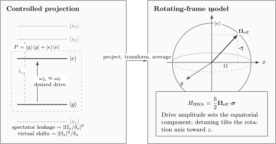
A two-level atom is obtained by a controlled projection, not by erasing the rest of the spectrum. Spectator couplings set leakage and virtual shifts. After the exact frame change and the RWA, drive amplitude and detuning form the effective Bloch rotation axis.

Detuning

Convention and physical meaning

This page defines

$$\Delta = \omega_0-\omega_L.$$

A red-detuned drive has $\omega_L<\omega_0$ and therefore $\Delta>0$. Some references define the negative of this quantity. Neither convention is more physical, but mixing them reverses the $z$ component of the rotating-frame Hamiltonian.

Detuning measures phase slip. In a frame rotating at $\omega_L$, the atomic coherence would rotate at $\omega_0-\omega_L$ without the transverse drive. Resonance means that the relevant phase slip vanishes after all shifts and frame choices have been included.

Bare versus effective detuning

The transition frequency in an experiment is seldom exactly the bare $\omega_0$. If the two selected levels acquire shifts $\delta E_e$ and $\delta E_g$, then

$$\Delta_{\mathrm{eff}}(t) = \omega_0 + \frac{ \delta E_e(t)-\delta E_g(t) }{ \hbar } - \dot\theta_L(t).$$

The differential shift can contain:

• static and ac Stark shifts;
• Zeeman shifts;
• collisional and mean-field shifts;
• trap-induced tensor shifts;
• recoil and motional sideband offsets;
• virtual shifts from spectator levels;
• the Bloch–Siegert correction;
• calibration offsets in the oscillator phase.

A resonance scan measures where the complete effective detuning vanishes, not automatically where a tabulated field-free frequency equals a nominal laser setting.

Motion and Doppler shift

For a traveling-wave phase

$$\theta_L(\mathbf R,t) = \omega_Lt - \mathbf k\mathbin{\cdot}\mathbf R(t) + \phi,$$

the phase rate seen by an atom is

$$\dot\theta_L = \omega_L - \mathbf k\mathbin{\cdot}\mathbf v.$$

With the detuning convention above,

$$\Delta_{\mathrm{eff}} = \omega_0-\omega_L + \mathbf k\mathbin{\cdot}\mathbf v + \delta\omega_{\mathrm{other}}.$$

The sign follows directly from the chosen optical phase. Writing the phase first is safer than memorizing a Doppler-detuning sign.

Quasienergy splitting

For constant parameters, define

$$\boldsymbol\Omega_{\mathrm{eff}} = \left( \Omega\cos\phi, \Omega\sin\phi, \Delta \right).$$

The RWA Hamiltonian has eigenvalue separation

$$\hbar\Omega_R, \qquad \Omega_R = \sqrt{ \Omega^2+\Delta^2 }.$$

This generalized frequency is the length of the effective rotation vector. It does not mean that detuning improves population transfer. Detuning increases the rotation rate while tilting the axis away from the equatorial plane, which generally reduces the maximum inversion from an initial energy eigenstate. The complete population formula is derived in Rabi Oscillations: First Encounter.

Inhomogeneous detuning

An ensemble may have a distribution of detunings because of velocity, position-dependent fields, unresolved sublevels, or oscillator noise. Every member can evolve unitarily while the ensemble-averaged coherence decays. That reversible inhomogeneous dephasing is conceptually distinct from irreversible single-particle decoherence.

Bloch-Sphere Representation

State and Bloch vector

In the ordered basis $(|e\rangle,|g\rangle)$, write

$$|\psi\rangle = c_e|e\rangle + c_g|g\rangle.$$

The pure-state density operator can be expressed as

$$\rho = |\psi\rangle\langle\psi| = \frac12 \left( I+\mathbf r\mathbin{\cdot}\boldsymbol\sigma \right),$$

where

$$\begin{aligned} r_x &= 2\operatorname{Re}(c_e^*c_g), \\ r_y &= 2\operatorname{Im}(c_e^*c_g), \\ r_z &= |c_e|^2-|c_g|^2. \end{aligned}$$

For a normalized pure state, $|\mathbf r|=1$. The chosen convention places $|e\rangle$ at the north pole and $|g\rangle$ at the south pole. The excited-state population is

$$P_e = \frac{1+r_z}{2}.$$

The Bloch vector omits the state’s global phase. Its azimuth records the relative phase between the two basis amplitudes.

Hamiltonian as a rotation axis

The RWA Hamiltonian is

$$H_{\mathrm{RWA}} = \frac{\hbar}{2} \boldsymbol\Omega_{\mathrm{eff}} \mathbin{\cdot} \boldsymbol\sigma.$$

The von Neumann equation gives

$$\dot{\mathbf r} = \boldsymbol\Omega_{\mathrm{eff}} \mathbin{\times} \mathbf r.$$

Thus:

• $\Omega$ sets the transverse rotation rate;
• $\phi$ chooses the equatorial direction of the rotation axis;
• $\Delta$ supplies its longitudinal component;
• the identity part of a Hamiltonian supplies no Bloch rotation.

On resonance with $\phi=0$, the axis lies along $+x$. A phase change of $\pi/2$ rotates the control axis to $+y$. Positive detuning tilts the axis toward $+z$ under this page’s convention.

Pulse phase is geometric control

Suppose two resonant pulses have equal area but phases $\phi_1$ and $\phi_2$. They rotate around different equatorial axes. Their actions generally do not commute, so the relative phase affects the final population even though each pulse has the same intensity.

This is the geometric basis of phase-sensitive spectroscopy and composite pulses. It is also why an oscillator phase reset must be modeled as a frame operation, not merely as a decorative change to a cosine.

Pure sphere versus Bloch ball

Unitary evolution preserves $|\mathbf r|$. Relaxation and dephasing generally move the state into the Bloch ball:

$$|\mathbf r| < 1.$$

Longitudinal relaxation changes population and transverse dephasing damps coherence. Those processes cannot be represented by a state vector obeying only the Hermitian Hamiltonian above. They require a density operator and an open-system generator. See the AMO Optical Bloch Equations for the workhorse dissipative dynamics and its observable dictionary; the open-system treatment owns the general Lindblad derivation.

Worked Model Reductions

A forbidden clock line can still be two level

Consider one isolated Zeeman component of the $^{40}\mathrm{Ca}^{+}$

$$4s\,{}^2S_{1/2} \longleftrightarrow 3d\,{}^2D_{5/2}$$

transition near $729\ \mathrm{nm}$. The transition is electric quadrupole E2 rather than E1. Once polarization, magnetic field, pulse bandwidth, and neighboring Zeeman components are controlled, the selected pair can still be described by

$$\begin{aligned} H_{\mathrm{RWA}} &= \frac{\hbar}{2} \left( \Delta\sigma_z + \Omega_{E2}\sigma_\phi \right), \\ \sigma_\phi &= \cos\phi\,\sigma_x + \sin\phi\,\sigma_y. \end{aligned}$$

Only the microscopic expression for $\Omega_{E2}$ changes. The two-state kinematics does not. This example separates the multipole approximation from the two-level approximation.

Raman coupling as an emergent two-state model

Let two long-lived states $|1\rangle$ and $|2\rangle$ couple to an intermediate state $|r\rangle$. In a suitable rotating frame, take

$$\begin{aligned} \frac{H}{\hbar} ={}& \Delta|r\rangle\langle r| \\ &+ \frac12 \left( \Omega_1|r\rangle\langle1| + \mathrm{h.c.} \right) \\ &+ \frac12 \left( \Omega_2|r\rangle\langle2| + \mathrm{h.c.} \right). \end{aligned}$$

When

$$|\Delta| \gg |\Omega_1|, \ |\Omega_2|, \ \Gamma_r,$$

the intermediate amplitude can remain small. To leading order, eliminating $|r\rangle$ gives

$$\frac{H_{\mathrm{eff}}}{\hbar} = - \frac{1}{4\Delta} \begin{pmatrix} |\Omega_1|^2 & \Omega_1^*\Omega_2 \\ \Omega_2^*\Omega_1 & |\Omega_2|^2 \end{pmatrix}$$

in the $(|1\rangle,|2\rangle)$ basis, before adding two-photon detuning. The diagonal entries are light shifts; the off-diagonal entries provide the effective Raman coupling.

The model is two level only after the parent three-level dynamics, spontaneous scattering, and approximation error have been checked. Different elimination procedures can disagree if inconsistent orders are mixed, which is why the systematic derivation belongs to Adiabatic Elimination.

A pulse can break an otherwise good reduction

Suppose the nearest unwanted line is separated by

$$\delta_s = 2\pi\times100\ \mathrm{MHz}.$$

A smooth microsecond pulse has a characteristic bandwidth near the megahertz scale and can be spectrally selective. A few-nanosecond pulse has bandwidth of order hundreds of megahertz, so the same atom, polarization, and target transition may no longer form a closed two-state system.

“This atom is two level” is therefore incomplete. A defensible statement is:

For these states, fields, pulse spectrum, preparation, observable, and timescale, spectator population and phase errors remain below the stated tolerance.

Scope and Limitations

Approximation ledger

The common driven two-level Hamiltonian often contains several logically independent reductions:

• Nonrelativistic matter. Retain an atomic or molecular $H_{\mathrm{at}}$; omit pair creation and large relativistic corrections; test that relevant energies are much smaller than $mc^2$.
• Multipole truncation. Retain E1, M1, E2, or another stated operator; omit higher spatial moments; test $ka$, symmetry, and target precision.
• Prescribed field. Retain a classical amplitude and phase; omit depletion, photon statistics, and atom–field entanglement; test that the field remains effectively classical.
• Two-state projection. Retain the $P$ subspace; omit spectator populations while incorporating or bounding virtual shifts; test coupling, detuning, and bandwidth.
• Rotating frame. Retain slow coordinates; omit nothing when every transformed term is kept.
• Rotating-wave approximation. Retain the co-rotating term; omit counter-rotating dynamics; test that slow scales are much smaller than $\omega_0+\omega_L$.
• Closed dynamics. Retain a Hermitian $H_2$; omit relaxation, dephasing, and loss; test that the experiment is short compared with the relevant decay times.

Failure of one row does not automatically imply failure of the others.

Multilevel degeneracy

If several states lie within the drive bandwidth, the correct retained space may be three dimensional or larger. This occurs for unresolved Zeeman manifolds, near-degenerate hyperfine states, lambda and ladder systems, and molecules with dense rotational or vibrational structure.

Dark states and coherent population trapping are intrinsically multilevel: their defining interference involves more than one coupling pathway. Compressing them prematurely into a two-state model can remove the effect one intends to explain.

Leakage and virtual errors are different

Small final spectator population does not prove the model was harmless. A spectator can be virtually occupied and return its population while leaving:

• a differential phase;
• an ac Stark shift;
• a modified Rabi frequency;
• an effective two-photon coupling;
• spontaneous scattering through a lossy intermediate state.

Population measurements alone may miss these coherent and incoherent errors.

Strong and ultrafast driving

When $\Omega$ becomes a substantial fraction of $\omega_0$, the counter-rotating term cannot be treated as a small correction. When a pulse contains only a few carrier cycles, “envelope,” “instantaneous phase,” and “near resonance” require careful definitions.

Strong fields can also mix remote atomic levels, ionize the atom, or make field-dependent basis states more natural than the original bare states.

Quantized radiation

A semiclassical two-level atom cannot describe:

• atom–field entanglement;
• vacuum Rabi oscillations;
• photon-number-dependent splittings;
• photon antibunching and photon correlations;
• collapse and revival from a photon-number distribution.

The matter subsystem may still have two internal states, but the joint Hilbert space is not two dimensional.

Motion and recoil

Internal two-state dynamics can be entangled with external motion. In trapped ions, recoil produces carrier and sideband transitions. In free atoms, momentum changes and Doppler shifts correlate internal state with motion. A model that traces over motion can show reduced internal coherence even when the total evolution is unitary.

Open-system closure

Spontaneous decay from $|e\rangle$ may return population to $|g\rangle$, to other internal states, or outside the detected manifold. Only the first case is a closed two-level decay channel. Branching to dark states requires at least a sink or an enlarged state space.

A Practical Reduction Workflow

1. Name the physical states. Include all quantum numbers needed to distinguish $|g\rangle$ and $|e\rangle$.
2. State the parent Hamiltonian. Identify whether the drive is E1, M1, E2, Raman, magnetic resonance, or another coupling.
3. Define $P$ and enumerate $Q$. List every spectator reachable under the actual polarization and field geometry.
4. Compute desired and unwanted matrix elements. Selection rules alone do not supply magnitudes.
5. Compare coupling, detuning, linewidth, and bandwidth. Estimate both real leakage and virtual shifts.
6. Fix conventions. State basis order, $\sigma_z$, optical phase, detuning sign, and the factor-of-two convention for $\Omega$.
7. Transform frames exactly. Retain the $-i\hbar R^\dagger\dot R$ term and display the counter-rotating contribution before dropping it.
8. Justify the RWA separately. Check fast-frequency and pulse-envelope scales.
9. Add environment and motion as needed. Compare pulse duration with relaxation, dephasing, recoil, and trap timescales.
10. Validate against an enlarged model. Increase the retained state space until the observable changes by less than the error budget.

Common Mistakes

Treating “two level” as an atomic property

The reduction depends on drive frequency, polarization, pulse shape, initial state, observable, and timescale. Changing any of these can open a spectator channel.

Confusing the frame change with the RWA

The unitary rotating-frame transformation is exact. Discarding the counter-rotating term is an additional approximation.

Losing a factor of two in the Rabi frequency

Some authors write the laboratory coupling as $\hbar\Omega\cos(\omega_Lt)\sigma_x$; others use $\hbar\Omega\cos(\omega_Lt)\sigma_x/2$. The same symbol then denotes different physical frequencies.

Quoting detuning without its sign convention

$\omega_0-\omega_L$ and $\omega_L-\omega_0$ are both common. A bare symbol $\Delta$ is ambiguous until defined.

Ignoring differential diagonal shifts

A common energy shift is dynamically irrelevant for a closed two-state system. A differential shift changes detuning and can dominate precision errors.

Assuming no leakage means no spectator effect

Virtual population can produce phase shifts and scattering while the final spectator population is nearly zero.

Using the pure-state sphere for dissipative data

Relaxation and dephasing require the Bloch ball and a density-operator equation. A shrinking experimental Bloch vector is not generated by a Hermitian two-state Hamiltonian.

Calling every effective pair a qubit

A useful qubit additionally needs preparation, universal or task-relevant control, readout, and error characterization. A spectroscopically isolated line is not automatically a practical qubit.

Further Connections

• Dipole Approximation controls the spatial field expansion that often supplies the coupling.
• Atomic Selection Rules helps enumerate allowed target and spectator channels.
• Transition Rates in Light–Matter Interaction connects projected matrix elements to perturbative absorption and emission rates.
• Rabi Oscillations: First Encounter solves the constant near-resonant model.
• Rabi Oscillations connects that solution to drive intensity, readout, experimental traces, and imperfect-model diagnostics.
• Ramsey Interferometry develops the separated-pulse phase measurement built from two-level rotations.
• Rabi and Ramsey Control treats pulse calibration in the presence of relaxation, dephasing, and control errors.
• Optical Bloch Equations extends the model to driven Markovian dynamics, saturation, scattering, and count predictions.
• Dressed States diagonalizes the effective Hamiltonian, tracks its mixing angle, and connects the classical drive to quantized atom–photon manifolds.
• Light–Matter Models distinguishes semiclassical Rabi, quantized-mode, and collective models.
• AMO Model Index compares the two-level reduction with Λ, optical Bloch, quantized-mode, and collective alternatives.

References

• L. Allen and J. H. Eberly, Optical Resonance and Two-Level Atoms, Dover, 1987 — standard semiclassical two-level dynamics, pulse area, and optical resonance.
• C. Cohen-Tannoudji, J. Dupont-Roc, and G. Grynberg, Atom–Photon Interactions: Basic Processes and Applications, Wiley, 1992 — atom–field matrix elements, rotating frames, Rabi dynamics, and dressed states.
• B. W. Shore, The Theory of Coherent Atomic Excitation, Wiley, 1990 — systematic multilevel and driven-atom treatment with explicit approximation structure.
• C. J. Foot, Atomic Physics, Oxford University Press, 2005 — atomic levels, resonance, selection rules, and experimental control context.
• I. I. Rabi, “Space Quantization in a Gyrating Magnetic Field,” Physical Review 51, 652–654 (1937), doi:10.1103/PhysRev.51.652 — foundational driven magnetic-resonance calculation.
• F. Bloch and A. Siegert, “Magnetic Resonance for Nonrotating Fields,” Physical Review 57, 522–527 (1940), doi:10.1103/PhysRev.57.522 — counter-rotating correction and the Bloch–Siegert shift.
• E. Brion, L. H. Pedersen, and K. Mølmer, “Adiabatic Elimination in a Lambda System,” Journal of Physics A 40, 1033–1043 (2007), doi:10.1088/1751-8113/40/5/011 — controlled effective two-state reduction and its error.
• K. Bergmann, H. Theuer, and B. W. Shore, “Coherent Population Transfer among Quantum States of Atoms and Molecules,” Reviews of Modern Physics 70, 1003–1025 (1998), doi:10.1103/RevModPhys.70.1003 — multilevel coherent control and why dark-state protocols are not primitive two-level dynamics.
• M. O. Scully and M. S. Zubairy, Quantum Optics, Cambridge University Press, 1997 — semiclassical and quantized-field two-level models, relaxation, and optical Bloch equations.

Exercises

1. Remove the common energy

Let

$$H_0 = E_e|e\rangle\langle e| + E_g|g\rangle\langle g|.$$

Using this page’s Pauli convention, rewrite $H_0$ as an identity term plus a traceless term. Show explicitly why the identity term cannot affect a population measurement in a closed two-state experiment.

Solution

Since

$$\begin{aligned} |e\rangle\langle e| &= \frac12(I+\sigma_z), \\ |g\rangle\langle g| &= \frac12(I-\sigma_z), \end{aligned}$$

we obtain

$$H_0 = \frac{E_e+E_g}{2}I + \frac{E_e-E_g}{2}\sigma_z.$$

With

$$\bar E = \frac{E_e+E_g}{2}, \qquad \omega_0 = \frac{E_e-E_g}{\hbar},$$

this is

$$H_0 = \bar E I + \frac{\hbar\omega_0}{2}\sigma_z.$$

The propagator factors because $I$ commutes with $\sigma_z$:

$$U_0(t) = e^{-i\bar Et/\hbar} \exp\!\left( - \frac{i\omega_0t}{2}\sigma_z \right).$$

The first factor multiplies every state amplitude by the same phase. For any projector $\Pi$,

$$\langle\psi| U_0^\dagger\Pi U_0 |\psi\rangle$$

is unchanged by that common phase. A differential diagonal shift, by contrast, changes the coefficient of $\sigma_z$ and therefore changes relative phase and detuning.

2. Spectator leakage and phase

An intended resonant transition has Rabi frequency $\Omega$. One spectator transition has

$$\Omega_s = 0.30\Omega, \qquad \delta_s = 20\Omega.$$

Estimate:

1. the maximum spectator population;
2. the spectator-induced shift using $\delta\omega_s\simeq|\Omega_s|^2/(4\delta_s)$;
3. the phase accumulated from that shift during a resonant $\pi$ pulse of duration $T_\pi=\pi/\Omega$.

Solution

The leakage estimate is

$$\begin{aligned} P_s^{\mathrm{max}} &\lesssim \left| \frac{\Omega_s}{\delta_s} \right|^2 \\ &= \left( \frac{0.30}{20} \right)^2 \\ &= 2.25\times10^{-4}. \end{aligned}$$

The virtual shift is

$$\begin{aligned} \delta\omega_s &\simeq \frac{ (0.30\Omega)^2 }{ 4(20\Omega) } \\ &= 1.125\times10^{-3}\Omega. \end{aligned}$$

During the $\pi$ pulse,

$$\begin{aligned} \delta\varphi_s &= \delta\omega_sT_\pi \\ &\simeq \left( 1.125\times10^{-3}\Omega \right) \frac{\pi}{\Omega} \\ &\simeq 3.53\times10^{-3}\ \mathrm{rad}. \end{aligned}$$

The population error is small, but the phase is a first-order quantity in the shift and may already matter in a precision phase measurement.

3. Derive the exact rotating-frame terms

Start from

$$H_{\mathrm{lab}} = \frac{\hbar\omega_0}{2}\sigma_z + \hbar\Omega \cos(\omega_Lt+\phi)\sigma_x$$

and

$$R(t) = e^{-i\omega_Lt\sigma_z/2}.$$

Derive $H_{\mathrm{rot}}$ before making the RWA. Identify which two terms are discarded by the approximation.

Solution

The rotating state satisfies

$$|\psi_{\mathrm{lab}}\rangle = R|\psi_{\mathrm{rot}}\rangle,$$

so

$$H_{\mathrm{rot}} = R^\dagger H_{\mathrm{lab}}R - i\hbar R^\dagger\dot R.$$

Because $R$ commutes with $\sigma_z$,

$$\begin{aligned} R^\dagger \frac{\hbar\omega_0}{2}\sigma_z R - i\hbar R^\dagger\dot R &= \frac{\hbar}{2} \left( \omega_0-\omega_L \right) \sigma_z \\ &= \frac{\hbar\Delta}{2}\sigma_z. \end{aligned}$$

Now use

$$\begin{aligned} \sigma_x &= \sigma_++\sigma_-, \\ \cos\theta &= \frac12 \left( e^{i\theta}+e^{-i\theta} \right). \end{aligned}$$

and

$$\begin{aligned} R^\dagger\sigma_+R &= e^{i\omega_Lt}\sigma_+, \\ R^\dagger\sigma_-R &= e^{-i\omega_Lt}\sigma_-. \end{aligned}$$

Multiplying the factors gives

$$\begin{aligned} H_{\mathrm{rot}} ={}& \frac{\hbar\Delta}{2}\sigma_z \\ &+ \frac{\hbar\Omega}{2} e^{-i\phi}\sigma_+ \\ &+ \frac{\hbar\Omega}{2} e^{i\phi}\sigma_- \\ &+ \frac{\hbar\Omega}{2} e^{i(2\omega_Lt+\phi)}\sigma_+ \\ &+ \frac{\hbar\Omega}{2} e^{-i(2\omega_Lt+\phi)}\sigma_- \end{aligned}$$

The last row is counter-rotating and is discarded by the RWA. The transformation itself discarded nothing.

4. Drive phase and initial motion

On resonance, let $\Omega>0$ and set $\phi=\pi/2$. An atom begins in $|g\rangle$, so its Bloch vector is $\mathbf r(0)=-\widehat{\mathbf z}$. Find the effective rotation axis and the initial direction $\dot{\mathbf r}(0)$.

Solution

On resonance $\Delta=0$, and

$$\boldsymbol\Omega_{\mathrm{eff}} = \left( \Omega\cos\phi, \Omega\sin\phi, 0 \right).$$

For $\phi=\pi/2$,

$$\boldsymbol\Omega_{\mathrm{eff}} = \Omega\widehat{\mathbf y}.$$

The Bloch equation gives

$$\begin{aligned} \dot{\mathbf r}(0) &= \boldsymbol\Omega_{\mathrm{eff}} \mathbin{\times} \mathbf r(0) \\ &= \Omega\widehat{\mathbf y} \mathbin{\times} \left( -\widehat{\mathbf z} \right) \\ &= -\Omega\widehat{\mathbf x}. \end{aligned}$$

The phase has rotated the control axis from $x$ to $y$. With the stated Bloch and cross-product conventions, the ground-state vector initially moves toward $-x$.

5. Detuning ledger for a moving atom

A traveling wave has phase

$$\theta_L = \omega_Lt-\mathbf k\mathbin{\cdot}\mathbf R(t).$$

The excited level also acquires a positive ac Stark shift $\delta E_e>0$, while the ground level is unshifted.

1. Derive the effective detuning.
2. State how motion with $\mathbf k\cdot\mathbf v>0$ and the positive excited-state shift change $\Delta_{\mathrm{eff}}$.

Solution

The oscillator phase rate along the trajectory is

$$\dot\theta_L = \omega_L-\mathbf k\mathbin{\cdot}\mathbf v.$$

The shifted transition frequency is

$$\omega_0' = \omega_0 + \frac{\delta E_e}{\hbar}.$$

Therefore

$$\begin{aligned} \Delta_{\mathrm{eff}} &= \omega_0'-\dot\theta_L \\ &= \omega_0-\omega_L + \mathbf k\mathbin{\cdot}\mathbf v + \frac{\delta E_e}{\hbar}. \end{aligned}$$

Under this page’s sign convention, both $\mathbf k\cdot\mathbf v>0$ and $\delta E_e>0$ increase the effective detuning. The result follows from the explicit phase and does not require a memorized Doppler sign.

6. Separate the approximations

For each case, identify which approximation is most directly threatened: the electric-dipole approximation, the two-level approximation, the RWA, or the closed-system approximation.

1. A narrow laser drives an isolated E2 clock transition weakly for $10\ \mathrm{ms}$.
2. A two-cycle E1 pulse has central frequency near an isolated optical line.
3. A weak resonant E1 drive is applied for many excited-state lifetimes.
4. A narrowband E1 drive addresses two Zeeman components separated by less than its Rabi frequency.

Solution

1. The electric-dipole truncation is inapplicable because the intended coupling is E2. The two-level approximation and RWA may still be excellent if the selected clock component is isolated and weakly driven.
2. A two-cycle pulse is broadband and its envelope changes on the carrier timescale. The RWA is threatened, and the bandwidth can also threaten the two-level approximation. E1 spatial coupling may remain valid.
3. The closed-system approximation fails because spontaneous emission accumulates. Weak drive and good spectral isolation do not remove dissipation.
4. The two-level approximation fails because both Zeeman components belong in the retained subspace. The E1 and RWA assumptions can remain valid.

The cases demonstrate that the four approximations are logically independent.

7. Eliminate a Raman intermediate state

For amplitudes $(c_1,c_2,c_r)$, suppose

$$\begin{aligned} i\dot c_1 &= \frac{\Omega_1^*}{2}c_r, \\ i\dot c_2 &= \frac{\Omega_2^*}{2}c_r, \\ i\dot c_r &= \Delta c_r + \frac{\Omega_1}{2}c_1 + \frac{\Omega_2}{2}c_2. \end{aligned}$$

Assume $|\Delta|\gg|\Omega_1|,|\Omega_2|$ and set $\dot c_r\simeq0$ to leading order. Derive the effective Hamiltonian for $(c_1,c_2)$ and identify its diagonal and off-diagonal physics.

Solution

The stationary intermediate amplitude is

$$c_r \simeq - \frac{ \Omega_1c_1+\Omega_2c_2 }{ 2\Delta }.$$

Substitution gives

$$\begin{aligned} i\dot c_1 &= - \frac{|\Omega_1|^2}{4\Delta}c_1 - \frac{\Omega_1^*\Omega_2}{4\Delta}c_2, \\ i\dot c_2 &= - \frac{\Omega_2^*\Omega_1}{4\Delta}c_1 - \frac{|\Omega_2|^2}{4\Delta}c_2. \end{aligned}$$

Thus

$$\frac{H_{\mathrm{eff}}}{\hbar} = - \frac{1}{4\Delta} \begin{pmatrix} |\Omega_1|^2 & \Omega_1^*\Omega_2 \\ \Omega_2^*\Omega_1 & |\Omega_2|^2 \end{pmatrix}.$$

The diagonal terms are single-beam ac Stark shifts. The off-diagonal terms drive the effective Raman transition. If one writes the off-diagonal two-state Hamiltonian as

$$\frac{\hbar}{2} \left( \Omega_{\mathrm{eff}}|1\rangle\langle2| + \mathrm{h.c.} \right),$$

then

$$\Omega_{\mathrm{eff}} = - \frac{ \Omega_1^*\Omega_2 }{ 2\Delta }.$$

Spontaneous scattering and higher-order corrections still depend on the eliminated state, so the effective Hamiltonian is not the entire error model.

8. Reconstruct a Bloch vector

Consider

$$|\psi\rangle = \frac{\sqrt3}{2}|g\rangle + \frac{e^{i\pi/3}}{2}|e\rangle.$$

Using the ordered basis $(|e\rangle,|g\rangle)$, calculate $\mathbf r=(r_x,r_y,r_z)$, verify that the state is pure, and recover the excited-state probability from $r_z$.

Solution

The amplitudes are

$$c_e = \frac{e^{i\pi/3}}{2}, \qquad c_g = \frac{\sqrt3}{2}.$$

Their coherence is

$$c_e^*c_g = \frac{\sqrt3}{4}e^{-i\pi/3}.$$

Therefore

$$\begin{aligned} r_x &= 2\operatorname{Re}(c_e^*c_g) = \frac{\sqrt3}{4}, \\ r_y &= 2\operatorname{Im}(c_e^*c_g) = -\frac34, \\ r_z &= |c_e|^2-|c_g|^2 = -\frac12. \end{aligned}$$

The length is

$$\begin{aligned} |\mathbf r|^2 &= \frac{3}{16} + \frac{9}{16} + \frac{1}{4} \\ &= 1, \end{aligned}$$

so the state lies on the pure-state sphere. Finally,

$$P_e = \frac{1+r_z}{2} = \frac14,$$

which agrees with $|c_e|^2$.