Optical Bloch Equations

The optical Bloch equations describe a coherently driven two-level atom whose population and coherence also relax. They are the smallest model that simultaneously contains:

• Rabi rotation;
• detuning and optical phase;
• spontaneous emission;
• homogeneous pure dephasing;
• transient damping;
• a saturated continuous-wave steady state.

For the chapter convention

$$\Delta \equiv \omega_0-\omega_L,$$

and a drive phase chosen as zero, the workhorse equations are

$$\begin{aligned} \dot u &= -\Gamma_2u-\Delta v, \\ \dot v &= \Delta u-\Gamma_2v-\Omega w, \\ \dot w &= \Omega v-\Gamma(w+1). \end{aligned}$$

Here $w=\rho_{ee}-\rho_{gg}$ is the inversion, $u$ and $v$ are the two coherence quadratures, $\Gamma$ is the excited-state population-decay rate, and

$$\Gamma_2 = \frac{\Gamma}{2} + \gamma_\phi$$

is the transverse coherence-decay rate. These three coupled equations map directly to fluorescence, absorption, dispersion, scattering force, and power-broadened spectra.

Canonical Scope

Optical Bloch Equations in the open-systems volume owns the general Markovian derivation, relation to Lindblad dynamics, and unconditional-state interpretation. The present page adopts that structure as an AMO forward model and owns:

1. the chapter-wide detuning and Rabi-frequency translation;
2. the atomic population and polarization quadratures;
3. the steady fluorescence and scattering-rate dictionary;
4. saturation parameters and their relation to local intensity;
5. power-broadened response and detector models;
6. branching, spatial averaging, and multilevel failure diagnostics.

Other nearby canonical homes are:

• Two-Level Atom for selecting and projecting the physical states;
• Rabi Oscillations for closed-system pulse calibration and transient trace diagnostics;
• Line Shapes and Broadening for the taxonomy of homogeneous, inhomogeneous, Doppler, collision, and instrumental widths;
• Quantum Optical Master Equation for the system–reservoir assumptions behind radiative Markov models;
• Quantum-Jump Trajectories for dynamics conditioned on a detected photon record.
• Optical Bloch Equation Notebook for executable RK4 transients, analytic-versus-linear steady states, saturation and fluorescence curves, linewidth extraction, and physicality checks.

The same words and symbols often appear with opposite detuning signs or different factors of two. This page always starts from its Hamiltonian before interpreting a formula.

Density Matrix for a Two-Level Atom

Why amplitudes are not enough

A state vector describes one isolated coherent realization. Spontaneous emission entangles the atom with unobserved radiation, technical noise varies between runs, and experiments average over records. The reduced atomic state is therefore represented by

$$\rho = \begin{pmatrix} \rho_{ee} & \rho_{eg} \\ \rho_{ge} & \rho_{gg} \end{pmatrix}$$

in the ordered basis $\{|e\rangle,|g\rangle\}$.

Physical states satisfy

$$\begin{aligned} \rho^\dagger &= \rho, \\ \operatorname{Tr}\rho &= 1, \\ \rho &\ge 0. \end{aligned}$$

For a $2\times2$ density matrix, positivity implies

$$|\rho_{eg}|^2 \le \rho_{ee}\rho_{gg}.$$

The diagonal entries are populations. The off-diagonal entry $\rho_{eg}$ is the optical coherence: its magnitude sets the available dipole phase coherence, and its complex phase sets the polarization quadrature relative to the drive.

Bloch coordinates

Define

$$\begin{aligned} u &= \rho_{eg}+\rho_{ge}, \\ v &= i(\rho_{eg}-\rho_{ge}), \\ w &= \rho_{ee}-\rho_{gg}. \end{aligned}$$

Then

$$\rho = \frac12 \left( I+u\sigma_x+v\sigma_y+w\sigma_z \right),$$

and

$$\rho_{ee} = \frac{1+w}{2}.$$

The Bloch-vector length satisfies

$$u^2+v^2+w^2 \le 1.$$

Equality holds for a pure state. Dissipation generally moves the state inside the Bloch sphere.

What is measured

Different instruments couple to different components:

• state-selective detection measures $\rho_{ee}$ or $w$;
• absorptive response is associated with one coherence quadrature;
• dispersive phase response is associated with the other;
• total fluorescence from an ideal radiative channel is proportional to $\Gamma\rho_{ee}$;
• a time-resolved photon record requires a conditional model, not only the ensemble density matrix.

The optical Bloch equations provide $\rho(t)$. A detector model is still needed to predict recorded counts, voltage, or transmitted power.

Coherent Drive

Rotating-frame Hamiltonian

After the two-level reduction and rotating-wave approximation, choose the drive phase as the $x$ axis:

$$H_{\mathrm{RWA}} = \frac{\hbar}{2} \left( \Delta\sigma_z+\Omega\sigma_x \right).$$

This page uses

$$\Delta = \omega_0-\omega_L.$$

The canonical open-systems page uses the opposite detuning sign. Its equations agree after replacing $\Delta$ there by $-\Delta$ here.

For a drive phase $\phi$,

$$\Omega\sigma_x \longrightarrow \Omega\sigma_\phi,$$

where

$$\sigma_\phi = \cos\phi\,\sigma_x + \sin\phi\,\sigma_y.$$

A constant phase can define the transverse axes. Time-dependent phase noise cannot generally be removed once and forgotten.

Unitary density-matrix evolution

The coherent contribution is

$$\dot\rho_{\mathrm{coh}} = - \frac{i}{\hbar} \left[ H_{\mathrm{RWA}},\rho \right].$$

It preserves trace, eigenvalues, and purity. In Bloch form it gives

$$\dot{\mathbf r}_{\mathrm{coh}} = \boldsymbol\Omega_{\mathrm{eff}} \mathbin{\times} \mathbf r,$$

with

$$\boldsymbol\Omega_{\mathrm{eff}} = \left( \Omega,0,\Delta \right).$$

The drive does not directly create irreversible population transfer. It rotates population into coherence and coherence back into population.

Population–coherence feedback

For phase zero, the coherent pieces satisfy

$$\begin{aligned} \dot\rho_{ee}\big|_{\mathrm{coh}} &= - i\frac{\Omega}{2} \left( \rho_{ge}-\rho_{eg} \right), \\ \dot\rho_{eg}\big|_{\mathrm{coh}} &= - i\Delta\rho_{eg} - i\frac{\Omega}{2} \left( \rho_{gg}-\rho_{ee} \right). \end{aligned}$$

An incoherent population-only rate equation cannot reproduce this phase feedback. It becomes a controlled approximation only when coherence decays or averages away on an appropriately short timescale.

Spontaneous Emission

Spontaneous Emission derives the vacuum-mode continuum rate, Wigner–Weisskopf decay, dipole pattern, photon wavepacket, and environment dependence. This page takes the resulting rate $\Gamma$ as an input to driven dissipative dynamics.

Radiative jump operator

For an ideal closed transition,

$$\sigma_- = |g\rangle\langle e|$$

returns the excited state to the ground state. The dissipator is

$$\mathcal D[L]\rho = L\rho L^\dagger - \frac12 \left\{ L^\dagger L,\rho \right\}.$$

Spontaneous emission at rate $\Gamma$ contributes

$$\dot\rho_{\mathrm{sp}} = \Gamma\mathcal D[\sigma_-]\rho.$$

The jump term

$$\Gamma\sigma_-\rho\sigma_+$$

repopulates $|g\rangle$. The anticommutator terms remove excited amplitude. Keeping only a non-Hermitian loss Hamiltonian would miss repopulation and would not preserve the trace of the unconditional state.

Population and coherence decay

With no drive,

$$\dot\rho_{ee} = -\Gamma\rho_{ee},$$

so

$$\rho_{ee}(t) = \rho_{ee}(0)e^{-\Gamma t}.$$

The same channel damps optical coherence at half the population rate:

$$\dot\rho_{eg}\big|_{\mathrm{sp}} = - \frac{\Gamma}{2} \rho_{eg}.$$

Thus spontaneous emission alone gives

$$T_1 = \frac{1}{\Gamma}, \qquad T_2 = 2T_1.$$

The factor of two is a frequent source of linewidth mistakes.

Total rate versus detected record

The unconditional mean emission rate is

$$R_{\mathrm{sc}}(t) = \Gamma\rho_{ee}(t).$$

This is the total rate into the modeled radiative reservoir. A detector collects only selected solid angle, polarization, frequency, and time bins, and it has nonunit efficiency and background.

A single emitter produces discrete stochastic events. The smooth function $\Gamma\rho_{ee}(t)$ is an ensemble mean or repeated-run expectation.

Branching and dark states

Real excited states may decay into several lower states. If only a fraction $\beta$ returns to the selected $|g\rangle$, then the two-state subspace loses probability at rate

$$\frac{d}{dt} \operatorname{Tr}_{\{e,g\}}\rho = - \left( 1-\beta \right) \Gamma\rho_{ee}.$$

One must then:

• include the other lower states;
• add repumping and optical pumping;
• or explicitly use a trace-decreasing conditional subspace model.

Replacing $\Gamma$ by $\beta\Gamma$ everywhere is not correct: the excited state decays at the total rate $\Gamma$, while only the return flux to $|g\rangle$ carries the factor $\beta$.

Dephasing

Homogeneous pure dephasing

A minimal Markovian pure-dephasing term is

$$\dot\rho_{\phi} = \frac{\gamma_\phi}{2} \mathcal D[\sigma_z]\rho.$$

It leaves the populations unchanged and gives

$$\dot\rho_{eg}\big|_{\phi} = -\gamma_\phi\rho_{eg}.$$

Combining radiative decay and pure dephasing,

$$\Gamma_2 = \frac{\Gamma}{2} + \gamma_\phi.$$

Equivalently,

$$\frac{1}{T_2} = \frac{1}{2T_1} + \gamma_\phi.$$

Within this model,

$$T_2 \le 2T_1.$$

An experimental fit that violates this inequality signals inconsistent definitions, uncertainty, nonexponential behavior, or a model beyond these two Markovian channels.

What pure dephasing can represent

An effective $\gamma_\phi$ may summarize fast homogeneous fluctuations, collisions, elastic environment coupling, or white phase-diffusion noise. It should not automatically absorb:

• quasi-static detuning distributions;
• Doppler broadening;
• slow laser drift;
• spatially varying light shifts;
• unresolved neighboring lines;
• non-Markovian spectral diffusion.

Those effects can produce nonexponential coherence or inhomogeneous line shapes even when one exponential fit looks adequate over a short window.

Laser linewidth

A Lorentzian laser spectrum generated by ideal white frequency noise can often be represented by an added homogeneous coherence-decay rate. A Gaussian or structured oscillator spectrum generally cannot be reduced to one constant $\gamma_\phi$ without losing time dependence or correlations.

The distinction between $T_2$ and $T_2^*$ is developed in Decoherence Timescales.

Bloch-Vector Equations

Master equation

The AMO workhorse master equation is

$$\begin{aligned} \dot\rho ={}& - \frac{i}{\hbar} \left[ H_{\mathrm{RWA}},\rho \right] \\ &+ \Gamma\mathcal D[\sigma_-]\rho + \frac{\gamma_\phi}{2} \mathcal D[\sigma_z]\rho. \end{aligned}$$

Its independent density-matrix equations are

$$\begin{aligned} \dot\rho_{ee} ={}& -\Gamma\rho_{ee} - i\frac{\Omega}{2} \left( \rho_{ge}-\rho_{eg} \right), \\ \dot\rho_{eg} ={}& - \left( \Gamma_2+i\Delta \right)\rho_{eg} \\ &- i\frac{\Omega}{2} \left( \rho_{gg}-\rho_{ee} \right), \\ \rho_{gg} ={}& 1-\rho_{ee}. \end{aligned}$$

Hermiticity supplies $\rho_{ge}=\rho_{eg}^*$.

Real three-component form

In terms of $(u,v,w)$,

$$\begin{aligned} \dot u &= -\Gamma_2u-\Delta v, \\ \dot v &= \Delta u-\Gamma_2v-\Omega w, \\ \dot w &= \Omega v-\Gamma(w+1). \end{aligned}$$

The same equations can be written

$$\dot{\mathbf r} = A\mathbf r+\mathbf b,$$

where

$$A = \begin{pmatrix} -\Gamma_2 & -\Delta & 0 \\ \Delta & -\Gamma_2 & -\Omega \\ 0 & \Omega & -\Gamma \end{pmatrix},$$

and

$$\mathbf b = \begin{pmatrix} 0\\0\\-\Gamma \end{pmatrix}.$$

This is an affine flow. Spontaneous emission pulls the state toward the ground-state pole rather than toward the center of the Bloch ball.

Term-by-term interpretation

• $\Delta$ rotates the two coherence quadratures into each other.
• $\Omega$ rotates $v$ into population and population into $v$.
• $\Gamma_2$ contracts the transverse components.
• $\Gamma$ relaxes $w$ toward $-1$.
• The drive and relaxation together produce a nontrivial steady state.

Removing all rates recovers coherent Rabi rotation. Removing the drive gives exponential population and coherence decay.

Resonant transient

On resonance, $u$ decouples and the homogeneous $(v,w)$ dynamics has eigenvalues

$$\lambda_\pm = - \frac{\Gamma+\Gamma_2}{2} \pm \sqrt{ \frac{ (\Gamma-\Gamma_2)^2 }{ 4 } - \Omega^2 }.$$

In the underdamped regime,

$$\lambda_\pm = - \frac{\Gamma+\Gamma_2}{2} \pm i \sqrt{ \Omega^2 - \frac{ (\Gamma-\Gamma_2)^2 }{ 4 } }.$$

Thus a fast resonant Rabi trace has an approximate envelope rate

$$\Gamma_R \simeq \frac{\Gamma+\Gamma_2}{2}.$$

This transient diagnostic is developed more fully in Rabi Oscillations.

Numerical propagation

For piecewise-constant parameters,

$$\mathbf r(t) = \mathbf r_{\mathrm{ss}} + e^{At} \left[ \mathbf r(0)-\mathbf r_{\mathrm{ss}} \right].$$

For arbitrary pulses, integrate the master equation with the actual $\Omega(t)$, $\Delta(t)$, and $\phi(t)$. A solver should be checked against:

• trace preservation;
• Hermiticity;
• nonnegative density-matrix eigenvalues;
• the no-drive exponential limit;
• the closed-system limit;
• the analytic steady state.

Steady States

Algebraic solution

For constant drive, set all derivatives to zero and define

$$D \equiv \Gamma \left( \Delta^2+\Gamma_2^2 \right) + \Omega^2\Gamma_2.$$

The steady Bloch components are

$$\begin{aligned} u_{\mathrm{ss}} &= - \frac{ \Omega\Gamma\Delta }{ D }, \\ v_{\mathrm{ss}} &= \frac{ \Omega\Gamma\Gamma_2 }{ D }, \\ w_{\mathrm{ss}} &= - \frac{ \Gamma \left( \Delta^2+\Gamma_2^2 \right) }{ D }. \end{aligned}$$

Therefore

$$\rho_{ee}^{\mathrm{ss}} = \frac{ \Omega^2\Gamma_2 }{ 2D }.$$

The steady optical coherence is

$$\rho_{eg}^{\mathrm{ss}} = - \frac{ \Omega\Gamma \left( \Delta+i\Gamma_2 \right) }{ 2D }.$$

Every expression is even in detuning for the population but odd/even in the expected way for the dispersive/absorptive coherence quadratures.

Weak drive

When

$$\Omega^2\Gamma_2 \ll \Gamma \left( \Delta^2+\Gamma_2^2 \right),$$

the atom remains mostly in $|g\rangle$:

$$\rho_{ee}^{\mathrm{ss}} \simeq \frac{ \Omega^2\Gamma_2 }{ 2\Gamma \left( \Delta^2+\Gamma_2^2 \right) }.$$

The coherence is linear in $\Omega$:

$$\rho_{eg}^{\mathrm{ss}} \simeq - \frac{\Omega}{2} \frac{ \Delta+i\Gamma_2 }{ \Delta^2+\Gamma_2^2 }.$$

This is the linear-response regime. Population is second order in field amplitude, while polarization is first order.

Strong resonant drive

On resonance,

$$\rho_{ee}^{\mathrm{ss}} = \frac{ \Omega^2 }{ 2 \left( \Gamma\Gamma_2+\Omega^2 \right) }.$$

As $\Omega\to\infty$,

$$\rho_{ee}^{\mathrm{ss}} \longrightarrow \frac12.$$

A continuously driven closed two-level transition saturates at equal populations. This does not contradict a coherent $\pi$ pulse reaching $\rho_{ee}=1$: a pulse is a transient operation, while the continuous-wave steady state includes ongoing emission and re-excitation.

No extra pure dephasing

When $\gamma_\phi=0$,

$$\Gamma_2 = \frac{\Gamma}{2},$$

and

$$\rho_{ee}^{\mathrm{ss}} = \frac{ \Omega^2 }{ \Gamma^2+4\Delta^2+2\Omega^2 }.$$

The total steady scattering rate is then

$$R_{\mathrm{sc}} = \Gamma \frac{ \Omega^2 }{ \Gamma^2+4\Delta^2+2\Omega^2 }.$$

At very strong resonant drive,

$$R_{\mathrm{sc}} \longrightarrow \frac{\Gamma}{2}.$$

The atom cannot emit faster on average than one photon per two excited-state lifetimes in this ideal steady two-level model.

Thermal or pumped reservoirs

The equation

$$\dot w = \Omega v-\Gamma(w+1)$$

assumes zero-temperature relaxation to $|g\rangle$. Thermal excitation, incoherent pumping, or several reservoirs replace the target inversion $-1$ and can change the steady population beyond $1/2$.

That extension should be derived from explicit upward and downward rates, not inserted by changing the sign of $\Gamma$.

Saturation and Line Broadening

Detuning-dependent saturation

Define

$$s(\Delta) \equiv \frac{ \Omega^2\Gamma_2 }{ \Gamma \left( \Delta^2+\Gamma_2^2 \right) }.$$

Then

$$\rho_{ee}^{\mathrm{ss}} = \frac{ s(\Delta) }{ 2 \left[ 1+s(\Delta) \right] }.$$

The on-resonance parameter is

$$s_0 \equiv \frac{\Omega^2}{ \Gamma\Gamma_2 },$$

and

$$s(\Delta) = \frac{ s_0 }{ 1+\left( \Delta/\Gamma_2 \right)^2 }.$$

Authors also use $s$ for the on-resonance quantity. Always inspect the definition rather than the symbol alone.

Saturated line shape

The steady population can be written

$$\rho_{ee}^{\mathrm{ss}}(\Delta) = \frac{ s_0 }{ 2 \left[ 1+s_0+ \left( \Delta/\Gamma_2 \right)^2 \right] }.$$

The peak is

$$\rho_{ee}^{\mathrm{ss}}(0) = \frac{s_0}{ 2(1+s_0) }.$$

Its angular-frequency half-width at half maximum is

$$\Delta_{\mathrm{HWHM}} = \Gamma_2\sqrt{1+s_0},$$

so

$$\Delta_{\mathrm{FWHM}} = 2\Gamma_2\sqrt{1+s_0}.$$

Power broadening is therefore a property of the driven response, not an intrinsic linewidth of the unilluminated atom.

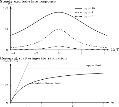
Top: increasing the resonant saturation parameter $s_0$ raises and broadens the steady excited-state response. Bottom: on resonance, $R_{\mathrm{sc}}/(\Gamma/2)=s_0/(1+s_0)$ approaches a finite plateau rather than growing indefinitely.

Ideal radiative transition

With no extra pure dephasing,

$$s_0 = \frac{2\Omega^2}{\Gamma^2}.$$

For an ideal closed electric-dipole transition driven by a plane wave with the dipole aligned to the polarization,

$$s_0 = \frac{I}{I_{\mathrm{sat}}},$$

where

$$I_{\mathrm{sat}} = \frac{ \pi h c\Gamma }{ 3\lambda^3 }.$$

This formula assumes:

• $\Gamma$ is an angular decay rate in $\mathrm{s^{-1}}$;
• the field-amplitude and Rabi-frequency convention used on this page;
• an ideal closed transition;
• the relevant dipole projection is maximal;
• no degeneracy or optical-pumping reduction.

Real atoms can attach Clebsch–Gordan factors, polarization dependence, branching, multilevel repumping, and convention-dependent numerical factors to a quoted saturation intensity.

Standard scattering-rate form

For the same ideal transition,

$$R_{\mathrm{sc}} = \frac{\Gamma}{2} \frac{ s_0 }{ 1+s_0+ \left( 2\Delta/\Gamma \right)^2 }.$$

This compact formula is ubiquitous in laser-cooling estimates. It is not universal for molecules, open transitions, coherent dark states, dense media, cavities, or structured reservoirs.

For one traveling-wave beam and one absorption–spontaneous-emission cycle, the mean dissipative force is approximately

$$\mathbf F_{\mathrm{sc}} = \hbar\mathbf k R_{\mathrm{sc}},$$

when spontaneous-emission recoil averages to zero. Multiple beams, directional emission, stimulated processes, and sub-Doppler polarization gradients require a larger model.

Radiation Pressure derives this mechanical force, its Doppler dependence, saturation ceiling, and recoil diffusion without duplicating the Bloch steady state.

Rabi frequency to intensity

For electric-dipole coupling,

$$\Omega = \frac{ \left| \langle e| \mathbf d\mathbin{\cdot} \widehat{\boldsymbol\epsilon} |g\rangle \right| \mathcal E_0 }{ \hbar },$$

and a plane wave has

$$I = \frac12 c\epsilon_0\mathcal E_0^2.$$

Thus $\Omega^2\propto I$, but the proportionality uses the local field and the actual polarization projection. Nominal laser power is not itself a Rabi frequency.

Broadening versus splitting

The formula

$$2\Gamma_2\sqrt{1+s_0}$$

describes one saturated steady-state population line in the ideal two-level model. When strong coherent coupling resolves dressed-state features, Autler–Townes structure, or the Mollow triplet, describing the signal as one power-broadened Lorentzian is no longer adequate.

Line Shapes and Broadening owns the broader comparison with Doppler, collision, transit-time, instrumental, and inhomogeneous effects.

Polarization, Fluorescence, and Counts

Absorptive and dispersive quadratures

In the weak-drive limit,

$$\begin{aligned} u_{\mathrm{ss}} &\simeq - \frac{ \Omega\Delta }{ \Delta^2+\Gamma_2^2 }, \\ v_{\mathrm{ss}} &\simeq \frac{ \Omega\Gamma_2 }{ \Delta^2+\Gamma_2^2 }. \end{aligned}$$

With the present phase convention, $u$ is odd in detuning and supplies the dispersive quadrature, while $v$ is even and supplies the absorptive quadrature. Rephasing the local oscillator rotates these labels.

The atomic dipole is proportional to $\rho_{eg}$ plus its conjugate in the laboratory frame. A transmission or phase-shift experiment therefore probes coherence, not simply excited-state population.

Fluorescence count model

For collection efficiency $\eta$, background count rate $b$, and detection window $[0,t_d]$, an ideal mean count is

$$\mu = b t_d + \eta \int_0^{t_d} dt\, \Gamma\rho_{ee}(t).$$

If events are independently detected and detector dead time is negligible, a starting count model is

$$n \sim \operatorname{Poisson}(\mu).$$

Under constant steady excitation,

$$\mu \simeq t_d \left( b+\eta R_{\mathrm{sc}} \right).$$

This model must be modified for antibunching-resolved time tags, detector dead time, afterpulsing, blinking, shelving, and background fluctuations. Photon Antibunching develops the post-click regression dynamics and detector-convolved correlation model.

Coherent and incoherent scattering

The total rate $\Gamma\rho_{ee}^{\mathrm{ss}}$ does not specify the optical spectrum. Resonance fluorescence contains:

• an elastically scattered coherent component linked to $|\langle\sigma_-\rangle|^2$;
• an inelastic component governed by two-time dipole correlations.

At strong drive, the inelastic spectrum can form the Mollow triplet. The one-time optical Bloch steady state supplies ingredients for that calculation, but not the spectrum by itself.

Transmission is a propagation problem

For a dilute optically thin sample, the single-atom coherence can be mapped to susceptibility and absorption. At appreciable optical depth, the field changes while propagating and drives different atoms with different amplitudes and phases.

Then one may need Maxwell–Bloch equations, radiative transfer, collective scattering, or a coupled-dipole model. Multiplying a single-atom scattering rate by atom number is not generally valid in a dense or optically thick sample.

Experimental Forward Models

Local intensity and ensemble averaging

Suppose atoms have density $n(\mathbf r)$ and the beam gives $\Omega(\mathbf r)$. A detector response has the schematic form

$$\begin{aligned} S(\Delta) = \int d^3r\, n(\mathbf r) \,\mathcal F\!\left[ \rho_{\mathrm{ss}} \left( \Omega(\mathbf r),\Delta \right) \right]. \end{aligned}$$

Because saturation is nonlinear,

$$\left\langle \rho_{ee}^{\mathrm{ss}}(I) \right\rangle \ne \rho_{ee}^{\mathrm{ss}} \left( \langle I\rangle \right)$$

in general. A Gaussian beam can therefore distort both the apparent contrast and line shape.

Motion and Doppler detuning

For velocity $\mathbf v$,

$$\Delta(\mathbf v) = \Delta_0 + \mathbf k\mathbin{\cdot}\mathbf v$$

for the stated sign convention, with $\mathbf k$ pointing along laser propagation and $\mathbf v$ the atomic laboratory velocity. The observed response averages the homogeneous optical Bloch result over the velocity distribution.

If velocity also changes transit time, intensity, or collection efficiency, the correct average is joint rather than a simple convolution.

Multilevel optical pumping

The two-level steady state assumes every decay returns to the addressed ground state and the drive couples only one transition. In a multilevel atom:

• different Zeeman components have different Rabi frequencies;
• spontaneous emission redistributes magnetic populations;
• dark states can form;
• repump fields add coherences and rates;
• light shifts move each component differently.

An “effective two-level” fit may summarize a narrow operating range, but its fitted $\Gamma$, $I_{\mathrm{sat}}$, or contrast need not be a microscopic atomic constant.

Pulsed versus steady-state data

The steady formulas apply only after transients have decayed. A pulse of duration comparable to $T_1$, $T_2$, or one Rabi period requires the time-dependent equations.

Useful checks are:

1. fit several pulse durations with shared rates;
2. vary power to separate $\Omega$ from $\Gamma_2$;
3. scan detuning to constrain line center and width;
4. calibrate readout independently;
5. inspect whether fitted rates change with the chosen time window.

Parameter identifiability

A single steady line can constrain combinations such as

$$s_0 = \frac{\Omega^2}{ \Gamma\Gamma_2 }$$

more directly than the three quantities separately. Independent lifetime, Rabi-frequency, or coherence measurements are needed to identify $\Gamma$, $\Omega$, and $\gamma_\phi$ individually.

A Reliable Workflow

1. Select the physical levels. List all nearby states and radiative branches.
2. State conventions. Write the Hamiltonian, detuning sign, drive phase, and factor multiplying $\Omega$.
3. List channels. Distinguish spontaneous decay, pure dephasing, leakage, incoherent pumping, and technical averaging.
4. Write the master equation. Do not begin from a memorized saturation curve.
5. Derive the observable. Population, polarization, fluorescence, force, and transmission are not interchangeable.
6. Choose transient or steady state. Compare the experimental duration with all relaxation eigenvalues.
7. Average last. Apply spatial, velocity, and noise distributions to the nonlinear response.
8. Fit counts with their statistics. Preserve Poisson or binomial variance and detector backgrounds.
9. Test limits. Recover closed Rabi dynamics, no-drive relaxation, weak linear response, and strong-drive saturation.
10. Enlarge the model when residuals are structured. Extra levels, time-dependent noise, propagation, and conditional records leave recognizable signatures.

Scope and Limitations

Markov approximation

Constant $\Gamma$ and $\gamma_\phi$ assume reservoir memory is short on the system timescale. Structured photonic environments, strong coupling, retardation, and slow spectral diffusion can violate this assumption.

Semiclassical drive

The driving field is prescribed. The equations do not describe depletion, atom–field entanglement, photon-number-dependent Rabi frequencies, or cavity backaction.

Rotating-wave approximation

Counter-rotating terms are omitted. Strong drive can produce Bloch–Siegert shifts and additional harmonics. The controlled approximation criteria live in Rotating-Wave Approximation.

Independent atoms

The single-atom equations omit dipole–dipole interactions, superradiance, subradiance, reabsorption, and cooperative shifts. These can matter at high density or in structured geometries.

Unconditional evolution

The density matrix averages over unobserved emission records. Continuous monitoring, feedback, heralding, and time-resolved conditional state estimation require stochastic trajectories or filtering equations.

Phenomenological dephasing

A fitted constant $\gamma_\phi$ is not a microscopic explanation. Its meaning depends on the timescale, protocol, and noise spectrum.

Common Mistakes

• Using the wrong detuning sign. Translate from the Hamiltonian before comparing coherence equations.
• Losing a factor of two in $\Omega$. Check whether the Hamiltonian contains $\hbar\Omega\sigma_x/2$.
• Setting $\Gamma_2=\Gamma$. Spontaneous emission alone gives $\Gamma_2=\Gamma/2$.
• Treating $T_2^*$ as homogeneous $T_2$. Static distributions do not generally belong in one Markovian $\gamma_\phi$.
• Expecting continuous-wave inversion. A closed two-level steady state approaches $\rho_{ee}=1/2$, not $1$.
• Replacing total decay by a branching decay. Total $\Gamma$ removes excited population; branching controls where it goes.
• Calling every broadened strong-drive line a Lorentzian. Resolved dressed structure requires a larger response model.
• Equating fluorescence with coherent polarization. They probe different density-matrix combinations.
• Using nominal power instead of local intensity. Beam geometry, polarization, and mode quality set $\Omega$.
• Averaging intensity before applying saturation. Nonlinear response and averaging do not commute.
• Interpreting a smooth master-equation curve as one photon record. Individual records are stochastic.

Further Connections

• Laser Nomenclature translates peak versus positive-frequency field amplitudes, $\Omega$ versus $\Omega/(2\pi)$, detuning sign, and ideal versus transition-specific saturation intensity.
• Line Shape Reference collects the HWHM, FWHM, lifetime, Doppler, collision, and power-broadening conventions used to compare this response with measured spectra.
• Rabi Oscillations develops the underdamped transient and pulse-calibration limits.
• Ramsey Interferometry uses the same coherence rates in a separated-pulse phase measurement.
• Magnetic Resonance Overview translates the equations into longitudinal and transverse magnetization, free-induction, and CW resonance language.
• Transition Rates in Light–Matter Interaction distinguishes finite-pulse probabilities, perturbative rates, and stimulated versus spontaneous channels.
• Spontaneous Emission derives the microscopic radiative channel represented here by $\sqrt{\Gamma}\sigma_-$.
• Amplitude-Damping Master Equation owns the general zero-temperature relaxation channel.
• Pure-Dephasing Master Equation owns the general phase-damping channel.
• Autler–Townes Splitting extends the weak-probe Bloch calculation to a strongly controlled three-state ladder and separates splitting from transparency.
• Electromagnetically Induced Transparency extends the coherence equations to a Λ dark state, transparent window, and slow-light response.
• Radiation Pressure turns the steady scattering rate into a momentum-transfer force and retains the recoil fluctuations omitted by the internal-state equations.
• AMO Model Index locates the optical Bloch equations within the hierarchy of closed, open, semiclassical, and quantized light–matter models.

References

• F. Bloch, “Nuclear Induction,” Physical Review 70, 460–474 (1946), doi:10.1103/PhysRev.70.460 — driven magnetization with longitudinal and transverse relaxation.
• R. P. Feynman, F. L. Vernon, Jr., and R. W. Hellwarth, “Geometrical Representation of the Schrödinger Equation for Solving Maser Problems,” Journal of Applied Physics 28, 49–52 (1957), doi:10.1063/1.1722572 — real three-component representation of two-state dynamics.
• B. R. Mollow, “Power Spectrum of Light Scattered by Two-Level Systems,” Physical Review 188, 1969–1975 (1969), doi:10.1103/PhysRev.188.1969 — strong-drive resonance-fluorescence spectrum.
• L. Allen and J. H. Eberly, Optical Resonance and Two-Level Atoms, Dover, 1987 — standard optical Bloch solutions, transients, and saturation.
• C. Cohen-Tannoudji, J. Dupont-Roc, and G. Grynberg, Atom–Photon Interactions: Basic Processes and Applications, Wiley, 1992 — driven atoms, radiative damping, dressed states, and fluorescence.
• M. O. Scully and M. S. Zubairy, Quantum Optics, Cambridge University Press, 1997 — density-matrix response, coherence, and resonance fluorescence.
• H. J. Carmichael, An Open Systems Approach to Quantum Optics, Springer, 1993 — master equations and conditioned photon trajectories.
• C. J. Foot, Atomic Physics, Oxford University Press, 2005 — atomic transitions, saturation, optical pumping, and experimental conventions.
• H. J. Metcalf and P. van der Straten, Laser Cooling and Trapping, Springer, 1999 — two-level scattering rates and radiation pressure.
• R. Loudon, The Quantum Theory of Light, 3rd ed., Oxford University Press, 2000 — optical coherence, spontaneous emission, and resonance fluorescence.

Exercises

1. Density-matrix positivity

For

$$\rho = \begin{pmatrix} p & c \\ c^* & 1-p \end{pmatrix},$$

derive the positivity condition on $c$. Express the purity in terms of the Bloch-vector length.

Solution

The trace is already one. Positivity requires

$$0\le p\le1$$

and a nonnegative determinant:

$$\det\rho = p(1-p)-|c|^2 \ge 0.$$

Therefore

$$|c|^2 \le p(1-p).$$

Writing

$$\rho = \frac12 \left( I+\mathbf r\mathbin{\cdot}\boldsymbol\sigma \right),$$

and using

$$\left( \mathbf r\mathbin{\cdot}\boldsymbol\sigma \right)^2 = |\mathbf r|^2I,$$

gives

$$\operatorname{Tr}\rho^2 = \frac12 \left( 1+|\mathbf r|^2 \right).$$

Thus $|\mathbf r|=1$ for a pure state and $|\mathbf r|<1$ for a mixed state.

2. Why coherence decays at half the population rate

Apply

$$\Gamma\mathcal D[\sigma_-]\rho$$

to a general two-level density matrix. Show that the channel contributes $-\Gamma\rho_{ee}$ to the excited population and $-\Gamma\rho_{eg}/2$ to the coherence.

Solution

Since

$$\sigma_+\sigma_- = |e\rangle\langle e|,$$

the excited diagonal element of the jump term vanishes:

$$\langle e| \sigma_-\rho\sigma_+ |e\rangle = 0.$$

The two anticommutator pieces each contribute $-\Gamma\rho_{ee}/2$, so

$$\dot\rho_{ee}\big|_{\mathrm{sp}} = -\Gamma\rho_{ee}.$$

For the off-diagonal element, the jump term again vanishes. Only the left anticommutator factor contributes:

$$\begin{aligned} \dot\rho_{eg}\big|_{\mathrm{sp}} &= - \frac{\Gamma}{2} \langle e| \left\{ |e\rangle\langle e|,\rho \right\} |g\rangle \\ &= - \frac{\Gamma}{2} \rho_{eg}. \end{aligned}$$

Population is a probability and decays at $\Gamma$; coherence contains one excited-state amplitude and decays at half that rate.

3. Solve the steady state

Starting from

$$\begin{aligned} 0 &= -\Gamma_2u-\Delta v, \\ 0 &= \Delta u-\Gamma_2v-\Omega w, \\ 0 &= \Omega v-\Gamma(w+1), \end{aligned}$$

derive $\rho_{ee}^{\mathrm{ss}}$.

Solution

The first and third equations give

$$u = - \frac{\Delta}{\Gamma_2}v,$$

and

$$w = \frac{\Omega}{\Gamma}v-1.$$

Insert these into the second equation:

$$\Omega = v \left[ \frac{ \Delta^2+\Gamma_2^2 }{ \Gamma_2 } + \frac{\Omega^2}{\Gamma} \right].$$

Therefore

$$v_{\mathrm{ss}} = \frac{ \Omega\Gamma\Gamma_2 }{ \Gamma \left( \Delta^2+\Gamma_2^2 \right) + \Omega^2\Gamma_2 }.$$

Because

$$\rho_{ee} = \frac{1+w}{2} = \frac{\Omega v}{2\Gamma},$$

one obtains

$$\rho_{ee}^{\mathrm{ss}} = \frac{ \Omega^2\Gamma_2 }{ 2 \left[ \Gamma \left( \Delta^2+\Gamma_2^2 \right) + \Omega^2\Gamma_2 \right] }.$$

4. Power-broadened width

Using

$$\rho_{ee}^{\mathrm{ss}}(\Delta) = \frac{ s_0 }{ 2 \left[ 1+s_0+ \left( \Delta/\Gamma_2 \right)^2 \right] },$$

find the HWHM and FWHM. What do they become when $\gamma_\phi=0$?

Solution

At resonance,

$$\rho_{ee}^{\mathrm{ss}}(0) = \frac{s_0}{ 2(1+s_0) }.$$

At half maximum, the denominator must double:

$$1+s_0+ \left( \frac{\Delta}{\Gamma_2} \right)^2 = 2(1+s_0).$$

Hence

$$|\Delta|_{\mathrm{HWHM}} = \Gamma_2\sqrt{1+s_0},$$

and

$$\Delta_{\mathrm{FWHM}} = 2\Gamma_2\sqrt{1+s_0}.$$

With no pure dephasing,

$$\Gamma_2 = \frac{\Gamma}{2}, \qquad s_0 = \frac{2\Omega^2}{\Gamma^2},$$

so

$$\Delta_{\mathrm{FWHM}} = \Gamma\sqrt{1+s_0}.$$

These widths are in angular-frequency units.

5. Saturation intensity estimate

For an ideal cycling transition with

$$\lambda = 780\ \mathrm{nm}, \qquad \frac{\Gamma}{2\pi} = 6.07\ \mathrm{MHz},$$

estimate

$$I_{\mathrm{sat}} = \frac{\pi h c\Gamma}{3\lambda^3}.$$

Express the result in $\mathrm{mW\,cm^{-2}}$.

Solution

The angular decay rate is

$$\begin{aligned} \Gamma &= 2\pi \left( 6.07\times10^6\ \mathrm{s^{-1}} \right) \\ &\simeq 3.81\times10^7\ \mathrm{s^{-1}}. \end{aligned}$$

Substitution gives

$$\pi h c\Gamma \simeq 2.38\times10^{-17}\ \mathrm{J\,m\,s^{-1}},$$

and

$$3\lambda^3 \simeq 1.42\times10^{-18}\ \mathrm{m^3}.$$

Thus

$$\begin{aligned} I_{\mathrm{sat}} &\simeq \frac{ 2.38\times10^{-17} }{ 1.42\times10^{-18} } \ \mathrm{W\,m^{-2}} \\ &\simeq 16.7\ \mathrm{W\,m^{-2}}. \end{aligned}$$

Since

$$1\ \mathrm{W\,m^{-2}} = 0.1\ \mathrm{mW\,cm^{-2}},$$

the result is

$$I_{\mathrm{sat}} \simeq 1.67\ \mathrm{mW\,cm^{-2}}.$$

This is the ideal two-level cycling value. A real transition’s polarization and angular-momentum factors must be checked.

6. Expected fluorescence counts

An ideal radiative transition has

$$\frac{\Gamma}{2\pi} = 6.0\ \mathrm{MHz}, \qquad s_0 = 2, \qquad \Delta = \frac{\Gamma}{2}.$$

The collection efficiency is $\eta=0.020$, the detection window is $t_d=100\ \mu\mathrm{s}$, and the mean background is one count per window. Find the expected total count.

Solution

The ideal scattering rate is

$$R_{\mathrm{sc}} = \frac{\Gamma}{2} \frac{ s_0 }{ 1+s_0+ \left( 2\Delta/\Gamma \right)^2 }.$$

Here

$$\left( \frac{2\Delta}{\Gamma} \right)^2 = 1,$$

so

$$\begin{aligned} R_{\mathrm{sc}} &= \frac{\Gamma}{2} \frac{2}{1+2+1} \\ &= \frac{\Gamma}{4}. \end{aligned}$$

Numerically,

$$R_{\mathrm{sc}} \simeq 9.42\times10^6\ \mathrm{s^{-1}}.$$

The detected signal mean is

$$\begin{aligned} \mu_{\mathrm{sig}} &= \eta R_{\mathrm{sc}}t_d \\ &= (0.020) (9.42\times10^6) (100\times10^{-6}) \\ &\simeq 18.8. \end{aligned}$$

Adding one background count gives

$$\mu_{\mathrm{tot}} \simeq 19.8.$$

This assumes steady excitation throughout the window and no detector dead time or optical pumping.

7. Added pure dephasing

Take $\Omega=\Gamma$ and $\gamma_\phi=\Gamma/2$.

1. Find $\Gamma_2$ and $s_0$.
2. Find the resonant steady excited population.
3. Find the power-broadened angular FWHM.
4. Compare with the no-pure-dephasing case at the same $\Omega$.

Solution

With added pure dephasing,

$$\Gamma_2 = \frac{\Gamma}{2} + \frac{\Gamma}{2} = \Gamma.$$

Therefore

$$s_0 = \frac{\Omega^2}{ \Gamma\Gamma_2 } = 1.$$

The resonant population is

$$\rho_{ee}^{\mathrm{ss}}(0) = \frac{1}{2(1+1)} = \frac14.$$

The FWHM is

$$\Delta_{\mathrm{FWHM}} = 2\Gamma\sqrt2.$$

Without pure dephasing,

$$\Gamma_2 = \frac{\Gamma}{2}, \qquad s_0 = 2,$$

so

$$\rho_{ee}^{\mathrm{ss}}(0) = \frac{2}{2(1+2)} = \frac13,$$

and

$$\Delta_{\mathrm{FWHM}} = \Gamma\sqrt3.$$

At fixed drive, added dephasing lowers the resonant excitation and broadens the line.

8. Branching leakage

An excited state decays at total rate $\Gamma$. A fraction $\beta$ returns to $|g\rangle$, while $1-\beta$ enters unmodeled dark states.

1. Write the population equations in the $\{|e\rangle,|g\rangle\}$ subspace with the drive off.
2. Show that the subspace trace decreases.
3. Explain why replacing $\Gamma$ by $\beta\Gamma$ in the closed two-level optical Bloch equations is wrong.

Solution

The excited population decays through every branch:

$$\dot\rho_{ee} = -\Gamma\rho_{ee}.$$

Only the selected branch repopulates $|g\rangle$:

$$\dot\rho_{gg} = \beta\Gamma\rho_{ee}.$$

Therefore

$$\begin{aligned} \frac{d}{dt} \left( \rho_{ee}+\rho_{gg} \right) &= - \Gamma\rho_{ee} + \beta\Gamma\rho_{ee} \\ &= - \left( 1-\beta \right) \Gamma\rho_{ee}. \end{aligned}$$

The missing probability occupies dark states outside the chosen subspace. Replacing $\Gamma$ by $\beta\Gamma$ would incorrectly lengthen the excited state’s total lifetime and its radiative coherence time. The correct model keeps total $\Gamma$ for loss from $|e\rangle$ and includes all destination states or an explicit trace-decreasing reduced subspace.