Optical Bloch Equation Notebook

A numerically stable trajectory is not necessarily a physical density matrix. An ODE solver can preserve the trace while producing a negative eigenvalue, can approach a steady state while using the wrong detuning sign, or can reproduce a saturated population while confusing emitted photons with detected counts. Dissipative two-level calculations need algebraic, numerical, and measurement-level checks.

This notebook supplies those checks for the optical Bloch equations. It computes:

1. weak, saturated, underdamped, detuned, and dephased transients;
2. exact no-drive population and coherence decay benchmarks;
3. steady states by both analytic formula and linear algebra;
4. saturation and total fluorescence rate;
5. power-broadened line shapes and full widths at half maximum (FWHM); and
6. RK4 refinement, Bloch-ball, and population-range diagnostics.

The retained headline results are:

Diagnostic	Computed value	What it tests
no-drive population-decay error	$9.27\times10^{-13}$	$\rho_{ee}(t)=e^{-\Gamma t}$
no-drive coherence-decay error	$2.27\times10^{-12}$	$u(t)=e^{-\Gamma_2t}$
largest medium-versus-fine RK4 population difference	$1.09\times10^{-8}$	transient time-step convergence
minimum refinement-difference ratio	$18.79$	fourth-order regime
analytic-versus-linear steady-state error	$2.22\times10^{-16}$	algebra and sign convention
population saturation-formula error	$1.11\times10^{-16}$	steady response identity
largest analytic-versus-bisection FWHM error	$2.10\times10^{-13}\Gamma$	independent linewidth extraction
largest retained Bloch-radius excess	$0$	density-matrix physicality

The zero Bloch-radius excess is a measured maximum after rounding, not a claim that classical RK4 is positivity preserving for arbitrary steps. The step-refinement test remains essential.

Run the investigation. The program and retained results below support the stated experiment. Follow Running an Experiment for environment and output-directory guidance. The recorded evidence applies to its stated parameters and environment.

Purpose and Canonical Scope

This page is the canonical home for the executable calculation that:

• propagates the optical Bloch equations with explicit fourth-order Runge–Kutta (RK4);
• validates population and coherence decay without a drive;
• compares computed transients at three internal step sizes;
• checks populations and the Bloch-ball condition along every retained trajectory;
• solves the continuous-wave steady state analytically and by a linear system;
• evaluates the saturation parameter and total emission rate;
• scans detuning to obtain power-broadened line shapes;
• extracts FWHM values by deterministic bisection; and
• exports every plotted curve, convergence record, and convention.

Neighboring pages retain distinct canonical responsibilities:

• Optical Bloch Equations owns the AMO derivation, parameter dictionary, saturation-intensity mapping, detector forward model, and experimental failure modes.
• Optical Bloch Equations in Open Systems owns the general Lindblad derivation and unconditional-state interpretation.
• Quantum Optical Master Equation owns the system–reservoir assumptions behind radiative Markov dynamics.
• Time-Dependent Two-Level Systems Notebook owns the preceding unitary, laboratory-frame, pulse-area, and Ramsey benchmarks.
• Spontaneous Emission owns the physical origin and atomic structure of radiative decay.
• Line Shapes and Broadening owns the taxonomy of homogeneous, inhomogeneous, Doppler, collision, and instrumental widths.
• Correlation Functions owns the two-time optical-coherence hierarchy and spectral-correlation definitions needed beyond a mean fluorescence rate.
• Quantum-Jump Trajectories owns dynamics conditioned on a photon record.

The present notebook verifies an unconditional two-state forward model. It does not duplicate the physical derivation or turn a mean emission rate into a photon-counting trajectory.

Reproducibility Contract

The executable artifact is a NumPy-only Python program:

• Download the program
• Driven transient data
• Saturation and fluorescence data
• Power-broadened line-shape data
• Linewidth data
• RK4 convergence data
• Machine-readable metadata and validation

Run the downloaded program from the folder where you saved it:

python optical-bloch-equation.py --output-dir results

The default run declares:

Item	Choice
language	Python 3
numerical dependency	NumPy
random numbers	none
population-decay rate	$\Gamma=1$
frequency unit	$\Gamma$
time unit	$1/\Gamma$
transient interval	$0\le\Gamma t\le15$
transient output samples	$601$
retained internal step	at most $0.005/\Gamma$
convergence steps	$0.04/\Gamma$, $0.02/\Gamma$, $0.01/\Gamma$
saturation samples	$251$
line-shape samples	$601$
linewidth drive samples	$80$
transient integrator	classical explicit RK4
linewidth root solver	deterministic bisection

There is no stochastic unraveling, hidden fit, adaptive tolerance, external ODE package, or plotting dependency. The program records all parameters, runtime versions, acceptance thresholds, analytic references, physical exclusions, and output filenames in JSON.

Claim boundary

The calculation is an optical Bloch solver and steady-response benchmark. It assumes:

• a valid two-state projection;
• a rotating-wave Hamiltonian;
• a semiclassical monochromatic drive;
• Markovian population decay;
• Markovian homogeneous pure dephasing; and
• an unconditional density matrix.

It omits multilevel branching, optical pumping, motion, Doppler averaging, spatial intensity variation, photon recoil, detector dead time, conditioned quantum jumps, non-Markovian noise, and field-correlation spectra. A species-specific prediction requires those assumptions to be reviewed against the transition and apparatus.

State and Convention

The basis, Pauli matrices, Rabi frequency, and detuning convention match the preceding coherent notebook:

$$\Delta=\omega_0-\omega_L,$$

with ordered basis $[|e\rangle,|g\rangle]$ and rotating-frame Hamiltonian

$$\frac{H}{\hbar} = \frac12 \left( \Delta\sigma_z+\Omega\sigma_x \right).$$

The general open-systems Optical Bloch page writes its local detuning as $\Delta_{\mathrm{open}}=\omega_L-\omega_0$. Therefore

$$\Delta=-\Delta_{\mathrm{open}}.$$

Translate that sign before comparing coherence quadratures. The steady population is even in detuning and can conceal a mismatch.

The density matrix is

$$\rho = \begin{pmatrix} \rho_{ee}&\rho_{eg}\\ \rho_{ge}&\rho_{gg} \end{pmatrix}, \qquad \operatorname{Tr}\rho=1.$$

Define Bloch coordinates

$$\begin{aligned} u &= \operatorname{Tr}(\rho\sigma_x) = 2\operatorname{Re}\rho_{eg}, \\ v &= \operatorname{Tr}(\rho\sigma_y) = -2\operatorname{Im}\rho_{eg}, \\ w &= \operatorname{Tr}(\rho\sigma_z) = \rho_{ee}-\rho_{gg}. \end{aligned}$$

Then

$$\rho = \frac12 \left( I+u\sigma_x+v\sigma_y+w\sigma_z \right)$$

and

$$\rho_{ee} = \frac{1+w}{2}.$$

For a qubit, Hermiticity and unit trace are not enough. Positivity requires

$$u^2+v^2+w^2\le1.$$

The notebook checks this Bloch-ball condition at every exported transient sample.

Ground-state initial condition

Every driven trace begins in

$$\mathbf r(0) = \begin{pmatrix} 0\\0\\-1 \end{pmatrix},$$

which represents $\rho(0)=|g\rangle\langle g|$. Separate no-drive tests begin in $|e\rangle$ or with $u=1$ to isolate population and coherence decay.

Optical Bloch Equations

The model equations are

$$\begin{aligned} \dot u &= -\Gamma_2u-\Delta v, \\ \dot v &= \Delta u-\Gamma_2v-\Omega w, \\ \dot w &= \Omega v-\Gamma(w+1), \end{aligned}$$

where

$$\Gamma_2 = \frac{\Gamma}{2} + \gamma_\phi.$$

Here:

• $\Gamma$ is the excited-state population-decay rate;
• $\gamma_\phi$ is the additional pure-dephasing rate;
• $\Gamma_2$ is the total transverse coherence-decay rate;
• $\Omega$ is the RWA Rabi angular frequency; and
• $\Delta$ follows the declared positive-above-resonance convention.

The equations can be written as an affine linear system

$$\dot{\mathbf r} = A\mathbf r+\mathbf b,$$

with

$$A = \begin{pmatrix} -\Gamma_2&-\Delta&0\\ \Delta&-\Gamma_2&-\Omega\\ 0&\Omega&-\Gamma \end{pmatrix}$$

and

$$\mathbf b = \begin{pmatrix} 0\\0\\-\Gamma \end{pmatrix}.$$

The source term drives an undriven atom toward $w=-1$. Omitting it would describe damping toward the maximally mixed state, not spontaneous emission into a zero-temperature reservoir.

Master-equation origin

The corresponding model master equation is

$$\dot\rho = -\frac{i}{\hbar}[H,\rho] + \Gamma\mathcal D[\sigma_-]\rho + \frac{\gamma_\phi}{2} \mathcal D[\sigma_z]\rho,$$

where

$$\mathcal D[L]\rho = L\rho L^\dagger - \frac12 \left\{ L^\dagger L,\rho \right\}.$$

The coefficient $\gamma_\phi/2$ is chosen so that the dephasing dissipator contributes $-\gamma_\phi\rho_{eg}$ to the optical coherence. Changing the collapse-operator normalization without changing the reported rate creates a common factor-of-two error.

The computational page starts from the real equations above. The open-systems pages own the derivation and complete-positivity conditions.

Numerical Propagator

The notebook uses classical explicit RK4. For

$$\dot{\mathbf r} = f(\mathbf r),$$

one step of size $h$ is

$$\begin{aligned} \mathbf k_1 &= f(\mathbf r_n), \\ \mathbf k_2 &= f\left( \mathbf r_n+\frac h2\mathbf k_1 \right), \\ \mathbf k_3 &= f\left( \mathbf r_n+\frac h2\mathbf k_2 \right), \\ \mathbf k_4 &= f\left( \mathbf r_n+h\mathbf k_3 \right), \end{aligned}$$

followed by

$$\mathbf r_{n+1} = \mathbf r_n + \frac h6 \left( \mathbf k_1+2\mathbf k_2+2\mathbf k_3+\mathbf k_4 \right).$$

For a smooth nonstiff problem at fixed final time, the global error is $O(h^4)$. RK4 does not exactly preserve the Bloch ball or the matrix exponential of the affine system.

Output and internal grids

The CSV output contains $601$ equally spaced times. Between adjacent output times, the propagator takes enough internal substeps that

$$h\le0.005/\Gamma.$$

The convergence calculation independently repeats every transient with

$$h_{\max} \in \left\{ 0.04,\ 0.02,\ 0.01 \right\}/\Gamma.$$

The output grid therefore controls the retained record, while the internal grid controls propagation error.

Why not exponentiate the constant matrix?

Because $A$ and $\mathbf b$ are constant in this benchmark, one could solve the affine system with a matrix exponential. RK4 is retained deliberately:

• it is a transparent baseline for later time-dependent drives and rates;
• refinement exposes a familiar global order;
• positivity must be checked rather than assumed; and
• the steady-state linear solve supplies an independent endpoint.

A production code may use exact segment exponentials, adaptive solvers, or specialized Lindblad integrators. It should keep equivalent validation layers.

No-Drive Benchmarks

Before testing driven behavior, the notebook removes the drive.

Excited-state population decay

For $\Omega=0$ and an initially excited atom,

$$\dot\rho_{ee} = -\Gamma\rho_{ee}.$$

Therefore

$$\rho_{ee}(t) = e^{-\Gamma t}.$$

Over $0\le\Gamma t\le10$, the retained RK4 trajectory differs from this analytic result by at most

$$9.27\times10^{-13}.$$

This test checks the affine source term as well as the mapping $\rho_{ee}=(1+w)/2$.

Coherence decay

With $\Omega=\Delta=0$, the $u$ quadrature obeys

$$\dot u=-\Gamma_2u.$$

For the test value

$$\frac{\gamma_\phi}{\Gamma}=0.75,$$

the exact result is

$$u(t) = e^{-1.25\Gamma t}.$$

The maximum retained difference is

$$2.27\times10^{-12}.$$

Population and coherence tests are separate because a code can implement $\Gamma$ correctly while using the wrong pure-dephasing normalization.

Driven Transients

The program exports five cases:

Case	$\Omega/\Gamma$	$\Delta/\Gamma$	$\gamma_\phi/\Gamma$	Purpose
resonant weak	$0.25$	$0$	$0$	monotonic weak excitation
resonant saturated	$1$	$0$	$0$	moderate saturation
resonant oscillatory	$3$	$0$	$0$	damped Rabi motion
detuned	$1$	$1.5$	$0$	tilted steady response
dephased	$1$	$0.5$	$0.75$	added transverse decay

All begin in the ground state and run to $\Gamma t=15$. The largest excited population among all retained cases is

$$0.6890629153,$$

from the first overshoot of the strongly driven resonant trace. Every population remains in $[0,1]$, and no sampled Bloch vector exceeds unit radius.

Resonant damping eigenvalues

On resonance, $u$ decouples. Deviations of $(v,w)$ from steady state evolve with matrix

$$A_{vw} = \begin{pmatrix} -\Gamma_2&-\Omega\\ \Omega&-\Gamma \end{pmatrix}.$$

Its eigenvalues are

$$\lambda_\pm = -\frac{\Gamma+\Gamma_2}{2} \pm \sqrt{ \frac{(\Gamma-\Gamma_2)^2}{4} -\Omega^2 }.$$

Oscillatory damping occurs when

$$\Omega > \frac{|\Gamma-\Gamma_2|}{2}.$$

For pure radiative decay, $\Gamma_2=\Gamma/2$, so the threshold is

$$\Omega>\frac{\Gamma}{4}.$$

The damped angular frequency is then

$$\Omega_{\mathrm d} = \sqrt{ \Omega^2-\frac{\Gamma^2}{16} },$$

and the envelope decays at $3\Gamma/4$. Thus $\Omega/\Gamma=0.25$ lies at the critical boundary, while $\Omega/\Gamma=3$ displays a clear underdamped overshoot.

A damped trace is not one exponential

The observed population can contain:

• Liouvillian eigenmodes with different decay rates;
• an oscillatory pair;
• a nonzero saturated offset;
• detuning-induced phase shifts;
• state-preparation and readout offsets; and
• ensemble averages absent from this model.

Fitting

$$A e^{-t/T}\cos(\Omega t+\phi)+C$$

may be useful phenomenology, but its fitted $T$ is not automatically $T_1$, $T_2$, or one Liouvillian eigenvalue.

Continuous-Wave Steady State

For constant parameters, the steady state satisfies

$$A\mathbf r_{\mathrm{ss}} = -\mathbf b.$$

The code solves this $3\times3$ system with numpy.linalg.solve. It also evaluates the analytic solution. Define

$$D = \Gamma \left( \Delta^2+\Gamma_2^2 \right) + \Omega^2\Gamma_2.$$

Then

$$\begin{aligned} u_{\mathrm{ss}} &= - \frac{\Omega\Gamma\Delta}{D}, \\ v_{\mathrm{ss}} &= \frac{\Omega\Gamma\Gamma_2}{D}, \\ w_{\mathrm{ss}} &= - \frac{ \Gamma(\Delta^2+\Gamma_2^2) }{D}. \end{aligned}$$

The dispersive coordinate $u_{\mathrm{ss}}$ is odd in the declared detuning, while $v_{\mathrm{ss}}$ and $\rho_{ee}^{\mathrm{ss}}$ are even. The first program run intentionally failed when the analytic helper used the opposite sign for $u_{\mathrm{ss}}$; comparison with the linear solve exposed the convention error.

The excited-state population is

$$\rho_{ee}^{\mathrm{ss}} = \frac{\Omega^2\Gamma_2}{2D}.$$

Across every saturation sample and selected dephasing value, the maximum component difference between analytic and linear-solve Bloch vectors is

$$2.22\times10^{-16}.$$

Long-time transient check

The final point of each driven trajectory is compared with its analytic steady vector. The largest residual is

$$9.55\times10^{-5}.$$

This is much larger than the time-step error because $\Gamma t=15$ is finite. It measures remaining physical relaxation toward the asymptote, not propagation failure. Confusing finite-time settling error with numerical error is a common mistake.

Saturation

Define the detuning-dependent saturation parameter

$$s(\Delta) = \frac{ \Omega^2\Gamma_2 }{ \Gamma(\Delta^2+\Gamma_2^2) }.$$

Then

$$\rho_{ee}^{\mathrm{ss}} = \frac{s}{2(1+s)}.$$

The program verifies this scalar formula against the analytic and linear-system solutions over

$$0\le\frac{\Omega}{\Gamma}\le5$$

for

$$\frac{\gamma_\phi}{\Gamma} \in \{0,\ 0.5,\ 2\}.$$

The maximum population discrepancy is

$$1.11\times10^{-16}.$$

Ideal radiative transition

When $\gamma_\phi=0$,

$$\Gamma_2=\frac{\Gamma}{2}$$

and

$$s(\Delta) = \frac{ 2\Omega^2/\Gamma^2 }{ 1+4\Delta^2/\Gamma^2 }.$$

On resonance,

$$\rho_{ee}^{\mathrm{ss}} = \frac{\Omega^2} {\Gamma^2+2\Omega^2}.$$

Representative values are:

$\Omega/\Gamma$	$s(0)$	$\rho_{ee}^{\mathrm{ss}}$
$0.1$	$0.02$	$0.0098039$
$0.5$	$0.5$	$1/6$
$1$	$2$	$1/3$
$2$	$8$	$4/9$

As $\Omega/\Gamma\to\infty$,

$$\rho_{ee}^{\mathrm{ss}}\to\frac12.$$

Coherent driving cannot invert this ideal two-level steady state. It equalizes the two populations in the strong-drive limit.

Added pure dephasing

At fixed $\Omega$ and exact resonance,

$$s(0) = \frac{\Omega^2}{\Gamma\Gamma_2}.$$

Increasing $\gamma_\phi$ therefore reduces excitation at fixed drive. For $\Omega=\Gamma$:

$\gamma_\phi/\Gamma$	$\Gamma_2/\Gamma$	$\rho_{ee}^{\mathrm{ss}}$
$0$	$0.5$	$1/3$
$0.5$	$1$	$1/4$
$2$	$2.5$	$1/7$

This does not mean dephasing always “reduces the area” of every measured spectrum. Which quantity is held fixed and which observable is integrated must be specified.

Fluorescence Rate

For the collapse operator

$$L=\sqrt{\Gamma}\,\sigma_-,$$

the total mean jump rate is

$$\begin{aligned} R_{\mathrm{fl}} &= \operatorname{Tr} \left( L^\dagger L\rho \right) \\ &= \Gamma\rho_{ee}. \end{aligned}$$

Therefore

$$\frac{R_{\mathrm{fl}}^{\mathrm{ss}}}{\Gamma} = \rho_{ee}^{\mathrm{ss}} = \frac{s}{2(1+s)}.$$

The normalized saturation and fluorescence curves in the figure are the same quantity. In physical units, the strong-drive ceiling is

$$R_{\mathrm{fl}}^{\mathrm{ss}} \longrightarrow \frac{\Gamma}{2}.$$

Total emission is not detected counts

For one observed channel, a simple count model is

$$R_{\mathrm{det}} = \eta_{\mathrm{sys}}\,b\,\Gamma\rho_{ee} + R_{\mathrm{bg}},$$

where:

• $b$ is the branching fraction into the counted optical channel;
• $\eta_{\mathrm{sys}}$ includes solid angle, optics, filtering, and detector efficiency; and
• $R_{\mathrm{bg}}$ is the background rate.

Detector dead time, afterpulsing, binning, and thresholding can require a nonlinear forward model. The notebook exports $R_{\mathrm{fl}}/\Gamma$, not laboratory counts per second.

Mean rate is not a spectrum

The equal-time jump rate uses $\rho_{ee}$. A resonance-fluorescence spectrum requires a two-time field correlation such as

$$G^{(1)}(\tau) \propto \left\langle \sigma_+(t+\tau)\sigma_-(t) \right\rangle_{\mathrm{ss}},$$

followed by a Fourier transform. Antibunching uses a second-order correlation. Neither follows from the mean rate alone. The quantum regression theorem or a trajectory calculation supplies the additional information.

Power-Broadened Line Shapes

At fixed $\Omega$, $\Gamma$, and $\Gamma_2$, the steady population is

$$\rho_{ee}^{\mathrm{ss}}(\Delta) = \frac{ \Omega^2\Gamma_2 }{ 2 \left[ \Gamma(\Delta^2+\Gamma_2^2) + \Omega^2\Gamma_2 \right] }.$$

It is an even Lorentzian in angular detuning for this homogeneous two-state model. The notebook scans

$$-6\le\frac{\Delta}{\Gamma}\le6$$

for

$$\frac{\Omega}{\Gamma} \in \{0.1,\ 0.5,\ 1,\ 2\}$$

with $\gamma_\phi=0$.

At every one of the $601$ detunings:

• the formula is compared with the linear steady-state solve; and
• opposite detunings are compared to verify reflection symmetry.

The maximum formula discrepancy is

$$7.89\times10^{-17},$$

and the largest reflection asymmetry is

$$2.22\times10^{-16}.$$

An odd population line shape under this model would therefore indicate a bug, a mismatched normalization, or physics beyond the assumed forward model.

Linewidth

The half-maximum detuning satisfies

$$\Delta_{1/2}^2 = \Gamma_2^2 + \frac{\Omega^2\Gamma_2}{\Gamma}.$$

Thus the angular-frequency FWHM is

$$\mathrm{FWHM} = 2 \sqrt{ \Gamma_2^2 + \frac{\Omega^2\Gamma_2}{\Gamma} }.$$

For pure radiative decay,

$$\mathrm{FWHM} = \Gamma \sqrt{ 1+2\frac{\Omega^2}{\Gamma^2} }.$$

The weak-drive width is $\Gamma$, while the width grows with drive because of saturation.

Independent numerical extraction

For each of $80$ drive values between

$$0.05\le\frac{\Omega}{\Gamma}\le4,$$

the program:

1. obtains the line centre from the linear steady-state solve;
2. sets the target to half that population;
3. brackets the positive-detuning crossing;
4. locates it by bisection; and
5. doubles the positive root.

The largest difference from the analytic FWHM is

$$2.10\times10^{-13}\Gamma.$$

The first and last extracted widths are:

$$\begin{aligned} \mathrm{FWHM}(0.05\Gamma) &= 1.0024968828\Gamma, \\ \mathrm{FWHM}(4\Gamma) &= 5.7445626465\Gamma. \end{aligned}$$

The small nonzero-drive correction explains why the first value is close to, but not exactly, $\Gamma$.

Width convention

This notebook reports:

• full width, not half width;
• angular frequency, not cycles per second;
• the width of steady excited population versus detuning;
• homogeneous two-state broadening; and
• no instrumental convolution.

Converting to ordinary frequency requires division by $2\pi$. A lifetime quoted as $1/\Gamma$ does not by itself identify whether an experimental paper reports angular HWHM, angular FWHM, frequency HWHM, or frequency FWHM.

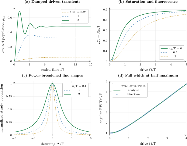
Unconditional two-state optical Bloch benchmarks with $\Gamma=1$. Panel (a) shows the transition from critically damped weak response to underdamped Rabi motion. Panel (b) gives $\rho_{ee}^{\mathrm{ss}}=R_{\mathrm{fl}}/\Gamma$ for three pure-dephasing rates. Panel (c) normalizes each steady line shape to expose power broadening. Panel (d) compares the analytic angular FWHM with roots extracted by bisection from the independent linear steady-state solve.

RK4 Convergence

For every transient case, define

$$\epsilon_{h,h/2} = \max_t \left| \rho_{ee}^{(h)}(t) - \rho_{ee}^{(h/2)}(t) \right|.$$

The retained table is:

Case	$h=0.04$ versus $0.02$	$h=0.02$ versus $0.01$	ratio
resonant weak	$6.31\times10^{-11}$	$3.34\times10^{-12}$	$18.88$
resonant saturated	$1.59\times10^{-9}$	$8.48\times10^{-11}$	$18.79$
resonant oscillatory	$2.06\times10^{-7}$	$1.09\times10^{-8}$	$18.86$
detuned	$6.82\times10^{-9}$	$3.63\times10^{-10}$	$18.80$
dephased	$2.67\times10^{-9}$	$1.42\times10^{-10}$	$18.86$

The exact values are exported in the convergence CSV. A fourth-order asymptotic error would suggest a ratio near $16$. The observed ratios are somewhat larger because:

• the diagnostic is a maximum over sampled time;
• leading error coefficients can partially cancel;
• the internal substep is shortened to land exactly on each output time; and
• higher-order terms are not negligible in an empirical three-grid ratio.

The important conclusions are:

• the ratios are stable and comfortably above the acceptance threshold of $10$;
• the largest medium-to-fine difference is only $1.09\times10^{-8}$; and
• qualitative damping and linewidth conclusions are many orders of magnitude larger than this numerical uncertainty.

Positivity audit

For each sampled Bloch vector, the program checks

$$r-1 = \sqrt{u^2+v^2+w^2}-1.$$

The largest positive excess is reported as zero at retained precision. It also checks

$$0\le\rho_{ee}\le1.$$

These checks should be repeated after changing step size, rates, or drive. Explicit RK methods are not generally completely positive maps.

Reading the Exported Data

Transient CSV

The file contains, for every case:

• $u$, $v$, and $w$;
• $\rho_{ee}$;
• $R_{\mathrm{fl}}/\Gamma$; and
• the common scaled time $\Gamma t$.

The fluorescence and population columns are intentionally both present. Their equality documents the normalization rather than asking a plotting script to infer it.

Saturation CSV

For each drive and pure-dephasing value, the file contains:

• on-resonance saturation parameter;
• population from the closed formula;
• population from the linear solve; and
• normalized fluorescence rate.

Line-shape CSV

For each drive, the file contains:

• formula population;
• linear-solve population; and
• population normalized to its own line-centre value.

Raw and normalized curves answer different questions. Normalization exposes width but hides the changing peak amplitude.

Linewidth CSV

Each row contains:

• drive strength;
• analytic FWHM;
• bisection-extracted FWHM;
• line-centre population; and
• line-centre fluorescence rate.

Convergence CSV

Each transient case records:

• physical parameters;
• all three maximum internal steps;
• both refinement differences;
• their ratio;
• final distance from steady state; and
• maximum Bloch-radius excess.

The last two quantities distinguish finite-duration settling and physicality from propagation convergence.

Validation Architecture

The notebook uses independent checks at several levels.

Equation-level checks

• no-drive population decay isolates $\Gamma$;
• no-drive coherence decay isolates $\Gamma_2$;
• the analytic steady state checks signs and factors;
• even population versus detuning checks symmetry.

Solver-level checks

• three-grid refinement checks global order;
• analytic decay checks absolute accuracy;
• final-state comparison checks the affine source and asymptote.

State-level checks

• population bounds;
• Bloch-ball positivity;
• real-valued coordinates; and
• finite values in every exported row.

Observable-level checks

• saturation formula;
• fluorescence ceiling;
• weak-drive linewidth;
• power-broadening trend; and
• independent half-maximum roots.

One check cannot replace the others. A solver can match the steady state while taking an inaccurate transient path, and a converged transient can faithfully solve the wrong equations.

Error Ledger

For comparison with an experiment, separate:

Layer	Representative uncertainty	Diagnostic
state projection	spectator levels and dark states	multilevel enlargement
Hamiltonian	$\Omega$, $\Delta$, polarization, phase	independent calibration
dissipator	branching, pumping, nonradiative decay	rate and channel model
Markov approximation	colored reservoir or technical noise	correlation-time test
time integration	truncation and stiffness	step refinement
physicality	negative density eigenvalues	Bloch radius or eigenspectrum
steady solver	sign or source error	analytic and linear comparison
ensemble	Doppler and intensity distribution	explicit averaging
photon mapping	branching and collection	detector forward model
line-shape mapping	convolution and frequency units	full fit ledger

The tiny RK4 error addresses only the time-integration row. It does not make the two-state Markov model exact.

Model discrepancy can dominate

Examples include:

• optical pumping into uncoupled Zeeman or hyperfine states;
• laser phase noise that is not white;
• transit-time effects;
• Doppler distributions;
• spatially varying $\Omega$;
• collisions;
• reabsorption and cooperative emission;
• detector saturation; and
• coherent propagation through an optically thick medium.

A physically larger model should be added because diagnostics demand it, not because the small model can be integrated to more digits.

Extending the Calculation

Time-dependent drive

Replace constant controls by

$$\Omega\to\Omega(t), \qquad \Delta\to\Delta(t).$$

Then compare with the unitary pulse-area benchmark as $\Gamma,\gamma_\phi\to0$. Record waveform interpolation and internal step placement.

Piecewise pulse sequences

Rabi, Ramsey, echo, and composite pulses can be simulated by changing $\Omega$, $\Delta$, and phase between segments. Finite-pulse detuning must remain active unless the instantaneous-pulse approximation is declared.

Multilevel branching

Introduce additional populations and coherences with channel-specific collapse operators. Validate:

• trace;
• positivity;
• branch-weighted total decay;
• population conservation including dark states; and
• recovery of the two-level result when unwanted branches vanish.

Motion and Doppler averaging

For a velocity distribution $f(v_z)$, use

$$\Delta(v_z) = \Delta_0-kv_z$$

and average the appropriate observable:

$$\overline{R}_{\mathrm{fl}} = \int dv_z\, f(v_z) R_{\mathrm{fl}}[\Delta(v_z)].$$

The average of steady rates is not the same as propagating one density matrix at an averaged detuning.

Radiation pressure

For one traveling wave and a closed transition, a simple mean force is

$$F = \hbar k\Gamma\rho_{ee}^{\mathrm{ss}}.$$

Multiple beams require their detunings, polarizations, and saturation to be combined consistently. The Laser Cooling Simulation Notebook owns the executable weak Doppler-force, friction, diffusion, and relaxation benchmark.

Photon trajectories

Unravel the same master equation into no-jump evolution and stochastic jumps. Ensemble-averaged trajectories should recover the unconditional density matrix within sampling uncertainty. Individual records can then test waiting times and antibunching.

Correlation functions

Use the quantum regression theorem to propagate operator-conditioned states and compute $G^{(1)}(\tau)$ or $g^{(2)}(\tau)$. Validate the zero-delay and long-delay limits before Fourier transforming.

Quantized cavity mode

Replace the prescribed classical drive by one quantized bosonic mode. The Cavity QED Simulation Notebook verifies the resulting Jaynes–Cummings dressed doublets, vacuum exchange, coherent-state photon-cutoff convergence, and a small unconditional Lindblad-loss model.

Stiff regimes

Large rate separations can make explicit RK4 inefficient or unstable. Implicit, exponential, or specialized master-equation methods may then be preferable. Solver choice should be based on eigenvalue scales and validated against a resolved reference.

Common Mistakes

Reversing the detuning sign

Steady population is even in $\Delta$, so it cannot expose the error. Inspect the odd dispersive quadrature $u_{\mathrm{ss}}$.

Omitting the affine source

Writing $\dot w=-\Gamma w$ relaxes toward $w=0$. Spontaneous emission into a zero-temperature reservoir requires $-\Gamma(w+1)$.

Double-counting coherence decay

Radiative population decay already contributes $\Gamma/2$ to $\Gamma_2$. Adding $\Gamma$ again as “decoherence” gives the wrong linewidth.

Confusing pure-dephasing conventions

The coefficient multiplying $\mathcal D[\sigma_z]$ depends on the collapse operator normalization. State the resulting off-diagonal decay rate.

Using one coarse RK4 run

A smooth damped curve can still have biased phase or peak height. Refine the internal step and compare the observable.

Assuming explicit RK4 preserves positivity

It does not generate a completely positive map for arbitrary $h$. Check density eigenvalues or Bloch radius.

Calling a finite-time endpoint the steady state

The residual at $\Gamma t=15$ is physical settling, not time-step error. Solve $A\mathbf r=-\mathbf b$ independently.

Reporting HWHM as FWHM

The half-maximum root is positive HWHM. The notebook doubles it and reports angular FWHM.

Mixing angular and cyclic frequency

Divide angular widths by $2\pi$ before reporting hertz.

Treating normalized line shapes as absolute response

Normalization erases peak suppression and total count scale.

Equating fluorescence with detector counts

Branching, collection, filtering, detector efficiency, background, and dead time intervene.

Equating mean fluorescence with the Mollow spectrum

A mean jump rate contains no two-time frequency information.

Calling $\Gamma^{-1}$ the coherence time

For pure radiative decay, $T_2=2/\Gamma$, not $1/\Gamma$. Pure dephasing reduces it further.

Applying the model to an open transition

Population can leak into dark states, invalidating the closed two-level steady state and the $\Gamma/2$ rate ceiling.

Exercises

Exercise 1: Bloch-ball positivity

Show that the eigenvalues of

$$\rho = \frac12 \left( I+\mathbf r\cdot\boldsymbol\sigma \right)$$

are $(1\pm|\mathbf r|)/2$. Deduce the positivity condition used by the notebook.

Solution

The Pauli identity gives

$$\left( \mathbf r\cdot\boldsymbol\sigma \right)^2 = |\mathbf r|^2I.$$

Therefore $\mathbf r\cdot\boldsymbol\sigma$ has eigenvalues $\pm|\mathbf r|$. Adding the identity and dividing by two gives

$$\lambda_\pm = \frac{1\pm|\mathbf r|}{2}.$$

Unit trace is automatic because

$$\lambda_++\lambda_-=1.$$

Both eigenvalues are nonnegative exactly when

$$|\mathbf r|\le1.$$

Thus the Bloch-ball test is equivalent to positivity for a Hermitian unit-trace $2\times2$ state. It would not be a sufficient general positivity test in higher dimension.

Exercise 2: no-drive relaxation

Set $\Omega=\Delta=0$. Solve the Bloch equations for arbitrary $u(0)$, $v(0)$, and $w(0)$.

Solution

The equations decouple:

$$\dot u=-\Gamma_2u, \qquad \dot v=-\Gamma_2v, \qquad \dot w=-\Gamma(w+1).$$

Therefore

$$\begin{aligned} u(t) &= u(0)e^{-\Gamma_2t}, \\ v(t) &= v(0)e^{-\Gamma_2t}, \\ w(t) &= -1+[w(0)+1]e^{-\Gamma t}. \end{aligned}$$

For an initially excited atom, $w(0)=1$, so

$$\rho_{ee}(t) = \frac{1+w(t)}{2} = e^{-\Gamma t}.$$

For pure radiative decay,

$$\Gamma_2=\frac{\Gamma}{2},$$

so coherence amplitude decays twice as slowly as excited population.

Exercise 3: solve the steady state

Starting from the three optical Bloch equations, derive $u_{\mathrm{ss}}$, $v_{\mathrm{ss}}$, and $w_{\mathrm{ss}}$ with the notebook’s detuning sign.

Solution

From the first steady equation,

$$u_{\mathrm{ss}} = -\frac{\Delta}{\Gamma_2}v_{\mathrm{ss}}.$$

The second gives

$$\begin{aligned} 0 &= \Delta u_{\mathrm{ss}} - \Gamma_2v_{\mathrm{ss}} - \Omega w_{\mathrm{ss}} \\ &= - \left( \frac{\Delta^2}{\Gamma_2} + \Gamma_2 \right) v_{\mathrm{ss}} - \Omega w_{\mathrm{ss}}. \end{aligned}$$

Thus

$$v_{\mathrm{ss}} = - \frac{\Omega\Gamma_2} {\Delta^2+\Gamma_2^2} w_{\mathrm{ss}}.$$

The third equation requires

$$\Omega v_{\mathrm{ss}} = \Gamma(w_{\mathrm{ss}}+1).$$

Substitution gives

$$w_{\mathrm{ss}} = - \frac{ \Gamma(\Delta^2+\Gamma_2^2) }{ \Gamma(\Delta^2+\Gamma_2^2) + \Omega^2\Gamma_2 }.$$

Defining the denominator as $D$, back-substitution yields

$$\begin{aligned} v_{\mathrm{ss}} &= \frac{\Omega\Gamma\Gamma_2}{D}, \\ u_{\mathrm{ss}} &= - \frac{\Omega\Gamma\Delta}{D}. \end{aligned}$$

The minus sign of $u_{\mathrm{ss}}$ follows from $\Delta=\omega_0-\omega_L$ and the stated definition of $v$.

Exercise 4: resonant saturation

For $\gamma_\phi=\Delta=0$, calculate the steady population and total fluorescence rate at $\Omega=\Gamma$. What is their strong-drive limit?

Solution

For pure radiative decay,

$$\Gamma_2=\frac{\Gamma}{2}.$$

On resonance,

$$\rho_{ee}^{\mathrm{ss}} = \frac{\Omega^2} {\Gamma^2+2\Omega^2}.$$

At $\Omega=\Gamma$,

$$\rho_{ee}^{\mathrm{ss}} = \frac{\Gamma^2}{3\Gamma^2} = \frac13.$$

The total emission rate is

$$R_{\mathrm{fl}}^{\mathrm{ss}} = \Gamma\rho_{ee}^{\mathrm{ss}} = \frac{\Gamma}{3}.$$

As $\Omega\to\infty$,

$$\rho_{ee}^{\mathrm{ss}}\to\frac12, \qquad R_{\mathrm{fl}}^{\mathrm{ss}}\to\frac{\Gamma}{2}.$$

Detected counts remain smaller unless every emitted photon is recorded.

Exercise 5: power-broadened width

Derive the FWHM of $\rho_{ee}^{\mathrm{ss}}(\Delta)$ at fixed drive. Reduce the result for $\gamma_\phi=0$.

Solution

The line-centre denominator is

$$D_0 = \Gamma\Gamma_2^2+\Omega^2\Gamma_2.$$

At half maximum, the denominator doubles:

$$\Gamma(\Delta_{1/2}^2+\Gamma_2^2) + \Omega^2\Gamma_2 = 2D_0.$$

Therefore

$$\Gamma\Delta_{1/2}^2 = \Gamma\Gamma_2^2+\Omega^2\Gamma_2,$$

so

$$\Delta_{1/2} = \sqrt{ \Gamma_2^2 + \frac{\Omega^2\Gamma_2}{\Gamma} }.$$

The full width is twice the positive half-width:

$$\mathrm{FWHM} = 2\Delta_{1/2}.$$

For $\Gamma_2=\Gamma/2$,

$$\mathrm{FWHM} = \Gamma \sqrt{ 1+2\frac{\Omega^2}{\Gamma^2} }.$$

At $\Omega=4\Gamma$, this is

$$\Gamma\sqrt{33} \approx 5.74456\Gamma,$$

matching the numerical extraction.

Exercise 6: damping threshold

Derive the condition for oscillatory resonant transients. Evaluate the damped angular frequency and envelope decay rate when $\gamma_\phi=0$.

Solution

The resonant $(v,w)$ deviation matrix has eigenvalues

$$\lambda_\pm = - \frac{\Gamma+\Gamma_2}{2} \pm \sqrt{ \frac{(\Gamma-\Gamma_2)^2}{4} -\Omega^2 }.$$

They form a complex-conjugate pair when

$$\Omega > \frac{|\Gamma-\Gamma_2|}{2}.$$

The oscillation frequency is

$$\Omega_{\mathrm d} = \sqrt{ \Omega^2 - \frac{(\Gamma-\Gamma_2)^2}{4} },$$

and the envelope decay rate is

$$\frac{\Gamma+\Gamma_2}{2}.$$

For $\gamma_\phi=0$, $\Gamma_2=\Gamma/2$, giving

$$\Omega_{\mathrm d} = \sqrt{ \Omega^2-\frac{\Gamma^2}{16} }$$

and envelope rate $3\Gamma/4$. The critical drive is $\Omega=\Gamma/4$.

Exercise 7: RK4 refinement

If the leading global error is $C(t)h^4$, what refinement-difference ratio is expected for steps $h$, $h/2$, and $h/4$? Why need the measured ratio not equal it exactly?

Solution

At fixed time,

$$\begin{aligned} y_h-y_{h/2} &= Ch^4 \left( 1-\frac1{16} \right) + O(h^5), \\ y_{h/2}-y_{h/4} &= \frac{Ch^4}{16} \left( 1-\frac1{16} \right) + O(h^5). \end{aligned}$$

Therefore

$$\frac{|y_h-y_{h/2}|} {|y_{h/2}-y_{h/4}|} \to16.$$

The notebook takes a maximum over sampled times, and the time attaining the maximum can change with resolution. Landing exactly on output times changes some internal substeps. Higher-order error terms and cancellation also shift a finite-grid ratio. Values near and stably above the expected scale, together with a small finest difference, support the convergence claim.

Exercise 8: expected counts

An atom has $\Gamma=2\pi\times6\ \mathrm{MHz}$ and is driven on resonance at $\Omega=\Gamma$. A channel has branching fraction $b=0.8$, total detection efficiency $\eta_{\mathrm{sys}}=0.02$, and background $R_{\mathrm{bg}}=3.0\times10^3\ \mathrm{s}^{-1}$. Estimate the observed steady count rate in the ideal two-level model.

Solution

At $\Omega=\Gamma$ with no pure dephasing,

$$\rho_{ee}^{\mathrm{ss}}=\frac13.$$

The total emission rate is

$$R_{\mathrm{fl}} = \frac{\Gamma}{3} = \frac{2\pi(6.0\times10^6)}{3} \approx 1.2566\times10^7\ \mathrm{s}^{-1}.$$

The detected signal contribution is

$$\begin{aligned} R_{\mathrm{sig}} &= \eta_{\mathrm{sys}}bR_{\mathrm{fl}} \\ &= 0.02(0.8) \left( 1.2566\times10^7 \right) \\ &\approx 2.01\times10^5\ \mathrm{s}^{-1}. \end{aligned}$$

Adding background gives

$$R_{\mathrm{det}} \approx 2.04\times10^5\ \mathrm{s}^{-1}.$$

This estimate assumes no dead time, leakage, reabsorption, or collection variation.

Exercise 9: dephasing at fixed drive

At $\Omega=\Gamma$ and $\Delta=0$, compute the steady population for $\gamma_\phi/\Gamma=0$, $0.5$, and $2$. Explain why comparing the three values is a fixed-drive comparison rather than a fixed-saturation comparison.

Solution

On resonance,

$$s(0) = \frac{\Omega^2}{\Gamma\Gamma_2}, \qquad \Gamma_2 = \frac{\Gamma}{2}+\gamma_\phi.$$

For $\Omega=\Gamma$:

1. $\gamma_\phi=0$ gives $\Gamma_2=\Gamma/2$, $s=2$, and $\rho_{ee}=2/[2(3)]=1/3$.
2. $\gamma_\phi=\Gamma/2$ gives $\Gamma_2=\Gamma$, $s=1$, and $\rho_{ee}=1/4$.
3. $\gamma_\phi=2\Gamma$ gives $\Gamma_2=5\Gamma/2$, $s=2/5$, and $\rho_{ee}=(2/5)/[2(7/5)]=1/7$.

The drive amplitude $\Omega$ is held fixed while $\Gamma_2$ changes, so the saturation parameter changes. A fixed-$s$ comparison would increase $\Omega$ with $\sqrt{\Gamma_2}$ and would produce the same steady population by construction.

Reproducibility Checklist

Before extending or citing the result, preserve:

• basis order;
• definitions of $u$, $v$, and $w$;
• detuning sign;
• Rabi-frequency convention;
• $\Gamma$, $\gamma_\phi$, and $\Gamma_2$ normalization;
• affine source term;
• initial density matrix;
• output and internal grids;
• integrator and refinement ladder;
• positivity diagnostic;
• steady-state reference;
• linewidth and frequency-unit convention;
• fluorescence-versus-detection mapping;
• runtime and dependency versions; and
• physical exclusions.

The JSON artifact records each choice used here. A modified program should update its metadata and acceptance thresholds together with the equations.

The Reproducibility Benchmarks suite independently checks the resonant steady population $\rho_{ee}^{\mathrm{ss}}=1/3$ and folds this notebook’s analytic agreement, producer validations, artifact hashes, and runtime record into a versioned cross-notebook report.

References

1. F. Bloch, “Nuclear Induction,” Physical Review 70, 460–474 (1946), doi:10.1103/PhysRev.70.460.
2. R. P. Feynman, F. L. Vernon, Jr., and R. W. Hellwarth, “Geometrical Representation of the Schrödinger Equation for Solving Maser Problems,” Journal of Applied Physics 28, 49–52 (1957), doi:10.1063/1.1722572.
3. G. Lindblad, “On the Generators of Quantum Dynamical Semigroups,” Communications in Mathematical Physics 48, 119–130 (1976), doi:10.1007/BF01608499.
4. V. Gorini, A. Kossakowski, and E. C. G. Sudarshan, “Completely Positive Dynamical Semigroups of N-Level Systems,” Journal of Mathematical Physics 17, 821–825 (1976), doi:10.1063/1.522979.
5. B. R. Mollow, “Power Spectrum of Light Scattered by Two-Level Systems,” Physical Review 188, 1969–1975 (1969), doi:10.1103/PhysRev.188.1969.
6. L. Allen and J. H. Eberly, Optical Resonance and Two-Level Atoms, Wiley (1975); Dover reprint (1987).
7. C. Cohen-Tannoudji, J. Dupont-Roc, and G. Grynberg, Atom–Photon Interactions: Basic Processes and Applications, Wiley (1992).
8. M. O. Scully and M. S. Zubairy, Quantum Optics, Cambridge University Press (1997).
9. H. J. Carmichael, An Open Systems Approach to Quantum Optics, Springer (1993), doi:10.1007/978-3-540-47620-7.
10. C. J. Foot, Atomic Physics, Oxford University Press (2005).
11. H. J. Metcalf and P. van der Straten, Laser Cooling and Trapping, Springer (1999), doi:10.1007/978-1-4612-1470-0.
12. E. Hairer, S. P. Nørsett, and G. Wanner, Solving Ordinary Differential Equations I: Nonstiff Problems, 2nd revised ed., Springer (1993), doi:10.1007/978-3-540-78862-1.