Wave-Packet Scattering Notebook

A time-dependent scattering animation can look persuasive while its transmission probability is wrong. Norm conservation does not detect an unresolved barrier, a premature measurement, periodic wraparound, or comparison with the wrong plane-wave quantity. This notebook turns the animation into a controlled numerical experiment.

A Gaussian packet approaches an exactly solvable rectangular barrier from the left. The state is propagated with a unitary split-step Fourier method. At late time, regional norms are compared with an independent benchmark obtained by averaging the exact stationary transmission coefficient over the packet’s momentum distribution.

The canonical Wave Packets and Scattering page owns the relation between localized packets and stationary scattering amplitudes. Rectangular Barrier Tunneling owns the matching derivation. This page owns the propagation algorithm, parameter study, convergence evidence, failure modes, and reproducibility record.

Run the investigation. The program and retained results below support the stated experiment. Follow Running an Experiment for environment and output-directory guidance. The recorded evidence applies to its stated parameters and environment.

Physical Problem

Use dimensionless units

$$\hbar=m=1$$

and solve

$$i\frac{\partial\psi}{\partial t} = \left[ -\frac12\frac{\partial^2}{\partial x^2} + V(x) \right] \psi.$$

The barrier is centered at the origin:

$$V(x) = \begin{cases} V_0, & |x|<a/2,\\ 0, & |x|>a/2. \end{cases}$$

The reported calculation uses

$$V_0=1, \qquad a=2.$$

The initial state is the normalized Gaussian

$$\begin{aligned} \psi(x,0) ={}& \left( \frac{1}{2\pi\sigma_x^2} \right)^{1/4} \\ &\times \exp\!\left[ -\frac{(x-x_0)^2}{4\sigma_x^2} + ik_0x \right]. \end{aligned}$$

Its position and momentum standard deviations are

$$\Delta x = \sigma_x, \qquad \Delta k = \frac{1}{2\sigma_x}.$$

For the production run,

$$x_0=-80, \qquad \sigma_x=10, \qquad k_0=1.$$

The central kinetic energy is

$$E_0 = \frac{k_0^2}{2} = \frac12 < V_0,$$

so the central plane-wave component is in the tunneling regime. The packet has negligible negative-momentum weight, approximately $3\times10^{-32}$ on the reported grid.

Independent Analytic Benchmark

For $0<E<V_0$, the exact plane-wave transmission coefficient is

$$T(E) = \left[ 1 + \frac{ V_0^2\sinh^2(\kappa a) }{ 4E(V_0-E) } \right]^{-1},$$

where

$$\kappa = \sqrt{2(V_0-E)}.$$

The corresponding trigonometric expression is used for $E>V_0$. The matching calculation is not repeated here; it belongs to Rectangular Barrier Tunneling.

At the central wavenumber,

$$T(k_0) = 0.0706508248532.$$

That is not the exact target for a packet of finite bandwidth. If $A(k)$ is the normalized initial momentum amplitude, the packet benchmark is

$$P_{\mathrm T}^{\mathrm{spec}} = \int_0^\infty |A(k)|^2T(k)\,dk.$$

For the reported packet,

$$P_{\mathrm T}^{\mathrm{spec}} = 0.0719492847010.$$

The difference from $T(k_0)$ is about $1.30\times10^{-3}$, much larger than the final numerical propagation error. Comparing the simulation only with $T(k_0)$ would therefore misidentify a physical bandwidth effect as a numerical error.

Split-Step Fourier Propagation

Write the Hamiltonian as

$$H = T+V, \qquad T = -\frac12\frac{\partial^2}{\partial x^2}.$$

The symmetric second-order step is

$$\begin{aligned} U_{\mathrm S}(\Delta t) ={}& e^{-iV\Delta t/2} e^{-iT\Delta t} e^{-iV\Delta t/2} \\ &+ O(\Delta t^3) \end{aligned}$$

per step, giving global $O(\Delta t^2)$ error when the required regularity and commutator bounds are controlled. The kinetic factor is diagonal in momentum space:

$$e^{-iT\Delta t} \longleftrightarrow e^{-ik^2\Delta t/2}.$$

One numerical step is therefore:

$$\begin{aligned} \psi^{(1)}(x) &= e^{-iV(x)\Delta t/2}\psi^n(x), \\ \widetilde\psi^{(2)}(k) &= e^{-ik^2\Delta t/2} \mathcal F[\psi^{(1)}](k), \\ \psi^{n+1}(x) &= e^{-iV(x)\Delta t/2} \mathcal F^{-1}[\widetilde\psi^{(2)}](x). \end{aligned}$$

Every multiplication is by a unit-modulus phase, and the orthonormal discrete Fourier transform is unitary. The represented finite-grid evolution therefore conserves the discrete norm up to floating-point roundoff.

That structural property is valuable but limited. It proves that the algorithm did not lose probability. It does not prove that the represented Hamiltonian, barrier, packet, or time step is accurate.

Periodic Grid and Barrier Placement

The FFT imposes periodic boundary conditions on a box of length $L$. Use cell-centered positions

$$x_j = \left( j-\frac N2+\frac12 \right) \Delta x, \qquad \Delta x = \frac LN.$$

For every grid in the convergence sequence, the barrier edges lie between cells and exactly $a/\Delta x$ cells represent the barrier. This avoids changing the effective barrier width irregularly as $N$ changes.

The production parameters are:

Quantity	Value
Box length $L$	$512$
Grid points $N$	$8192$
Spacing $\Delta x$	$0.0625$
Time step $\Delta t$	$0.0025$
Final time $t_f$	$190$
Time steps	$76000$
Barrier neighborhood	$
Boundary-monitor width	$25$ at each edge

The final reflected and transmitted packets remain far from the periodic boundaries. No absorber is used, so unitarity and regional accounting remain direct. The price is that propagation must stop before either outgoing packet wraps around the box.

Regional Probability Accounting

Choose $x_b=15$, well outside the barrier. Define

$$P_{\mathrm L}(t) = \int_{x<-x_b} |\psi(x,t)|^2\,dx,$$ $$P_{\mathrm{int}}(t) = \int_{|x|\leq x_b} |\psi(x,t)|^2\,dx,$$

and

$$P_{\mathrm R}(t) = \int_{x>x_b} |\psi(x,t)|^2\,dx.$$

These regions partition the grid, so

$$P_{\mathrm L} + P_{\mathrm{int}} + P_{\mathrm R} = \|\psi\|^2.$$

Before the collision, $P_{\mathrm L}$ is mostly incident probability and must not be called reflection. Only after the outgoing pieces separate and $P_{\mathrm{int}}$ becomes negligible may one identify

$$P_{\mathrm R}^{\mathrm{packet}} = P_{\mathrm L}(t_f), \qquad P_{\mathrm T}^{\mathrm{packet}} = P_{\mathrm R}(t_f).$$

Evolution

The density begins as a right-moving Gaussian, develops interference structure during the collision, and ends as spatially separated reflected and transmitted packets.

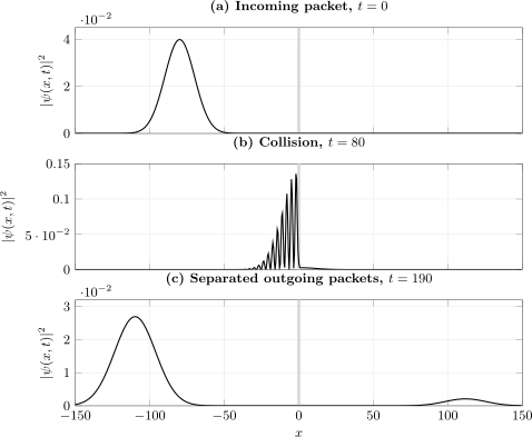
Density snapshots for $V_0=1$, $a=2$, $x_0=-80$, $k_0=1$, and $\sigma_x=10$. The shaded strip marks the barrier. The density scale changes between panels: packet probability is determined by the area under each outgoing branch, not by its peak height.

Selected regional probabilities are:

$t$	$P_{\mathrm L}$	$P_{\mathrm{int}}$	$P_{\mathrm R}$
$0$	$0.999999999960$	$4.02\times10^{-11}$	$1.05\times10^{-21}$
$60$	$0.682522753$	$0.317442019$	$3.52284\times10^{-5}$
$80$	$0.144997839$	$0.848267090$	$0.006735071$
$100$	$0.625072778$	$0.324185332$	$0.050741890$
$130$	$0.926534742$	$0.001601905$	$0.071863354$
$190$	$0.928055099$	$2.42\times10^{-12}$	$0.071944901$

The interaction probability peaks near $t=79.5$. At that time the labels incident, reflected, and transmitted are not separately meaningful. By $t=190$, the interaction remainder is negligible and the regional norms have stabilized.

Final Observable

The finest propagation gives

$$\begin{aligned} P_{\mathrm R}^{\mathrm{num}} &= 0.928055098720, \\ P_{\mathrm{int}}(t_f) &= 2.42\times10^{-12}, \\ P_{\mathrm T}^{\mathrm{num}} &= 0.071944901274. \end{aligned}$$

The accounted norm is

$$\begin{aligned} &P_{\mathrm R}^{\mathrm{num}}+P_{\mathrm{int}}(t_f)\\ &\qquad+P_{\mathrm T}^{\mathrm{num}}=0.999999999997. \end{aligned}$$

Against the independent packet-spectrum benchmark,

$$P_{\mathrm T}^{\mathrm{num}} - P_{\mathrm T}^{\mathrm{spec}} = -4.38343\times10^{-6}.$$

This discrepancy is about $6.1\times10^{-5}$ relative to the transmitted probability. It is small compared with the finite-bandwidth correction to $T(k_0)$.

Convergence Study

The rectangular barrier is discontinuous. Although the symmetric splitting is formally second order, the discontinuity populates high spatial frequencies and makes coarse time-step behavior less regular than a smooth-potential textbook estimate suggests. The observable must therefore be converged empirically.

Coordinated refinement

The main sequence halves $\Delta x$ and $\Delta t$ together while holding $L$ and $t_f$ fixed:

$$\Delta t = \frac{\Delta x}{25}.$$

| $N$ | $\Delta x$ | $\Delta t$ | $P_{\mathrm T}^{\mathrm{num}}$ | $|P_{\mathrm T}^{\mathrm{num}}-P_{\mathrm T}^{\mathrm{spec}}|$ | |---:|---:|---:|---:|---:| | $1024$ | $0.5$ | $0.02$ | $0.0713132071$ | $6.36078\times10^{-4}$ | | $2048$ | $0.25$ | $0.01$ | $0.0718504027$ | $9.88820\times10^{-5}$ | | $4096$ | $0.125$ | $0.005$ | $0.0719312085$ | $1.80762\times10^{-5}$ | | $8192$ | $0.0625$ | $0.0025$ | $0.0719449013$ | $4.38343\times10^{-6}$ |

The successive observed orders are approximately

$$2.69, \qquad 2.45, \qquad 2.04.$$

The sequence approaches second-order behavior, but this coordinated path alone cannot say whether space or time dominates.

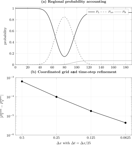
Panel (a) tracks left, interaction, and right regional probabilities. Panel (b) compares the propagated transmission with the exact momentum-weighted barrier coefficient under coordinated refinement. Exact norm conservation at every resolution does not prevent the coarsest transmitted probability from being wrong by more than $6\times10^{-4}$.

Time step at fixed grid

At fixed $N=4096$ and $\Delta x=0.125$:

$\Delta t$	$P_{\mathrm T}^{\mathrm{num}}$	Absolute Error
$0.01$	$0.0719211750$	$2.81097\times10^{-5}$
$0.005$	$0.0719312085$	$1.80762\times10^{-5}$
$0.0025$	$0.0719336018$	$1.56829\times10^{-5}$
$0.00125$	$0.0719341939$	$1.50908\times10^{-5}$

The error approaches a nonzero plateau. Reducing $\Delta t$ further cannot remove the spatial representation error at this $N$.

Box length at fixed resolution

Hold $\Delta x=0.0625$ and $\Delta t=0.0025$ fixed:

$L$	$N$	$P_{\mathrm T}^{\mathrm{num}}$	Final Edge Probability
$384$	$6144$	$0.07194490235$	$1.75\times10^{-5}$
$512$	$8192$	$0.07194490127$	$3.15\times10^{-16}$
$640$	$10240$	$0.07194490128$	$1.71\times10^{-16}$

The $L=512$ and $L=640$ transmissions agree to about $2\times10^{-12}$. The smaller box happens to give a similar integrated transmission at $t_f$, but probability has already entered the boundary-monitor region. It has no useful safety margin against periodic wraparound and is rejected.

Packet Bandwidth Is a Physical Control

For the Gaussian family,

$$\sigma_k = \frac{1}{2\sigma_x}.$$

Changing $\sigma_x$ changes the physical incoming state, not merely the numerical resolution. The exact spectrum averages are:

$\sigma_x$	$\sigma_k$	$P_{\mathrm T}^{\mathrm{spec}}$	$P_{\mathrm T}^{\mathrm{spec}}-T(k_0)$
$5$	$0.1$	$0.0759680480$	$5.31722\times10^{-3}$
$10$	$0.05$	$0.0719492847$	$1.29846\times10^{-3}$
$20$	$0.025$	$0.0709734396$	$3.22615\times10^{-4}$
$40$	$0.0125$	$0.0707313526$	$8.05277\times10^{-5}$

The packet result approaches $T(k_0)$ as the momentum distribution narrows. A wider packet samples the nonlinear energy dependence of $T(k)$ and should not be expected to reproduce the central plane-wave value.

Validation Ledger

Discrete norm

The production run satisfies

$$\max_t \left| \|\psi(t)\|^2-1 \right| < 4\times10^{-12}$$

over the recorded time series.

Regional accounting

At every recorded time, the three regional probabilities sum to the discrete norm within floating-point summation error.

Independent stationary benchmark

The late-time transmitted norm agrees with the exact momentum-weighted barrier coefficient within $4.4\times10^{-6}$ at the finest resolution.

Negative momentum

The initial negative-$k$ probability is below $4\times10^{-32}$, so essentially the entire packet approaches the barrier from the left.

Packet separation

The final interaction-region probability is below $3\times10^{-12}$. This is the operational check that the late-time regional norms may be interpreted as reflection and transmission.

Boundary clearance

The final probability in the outermost $25$ units on either side is below $4\times10^{-16}$ for $L=512$. The $L=640$ result confirms box-size stability.

Independent convergence axes

The calculation varies time step at fixed grid, box length at fixed spacing, packet width in the analytic benchmark, and space-time resolution along a coordinated refinement path.

Error Ledger

Source	Physical or Numerical?	Diagnostic	Control
Packet bandwidth	physical state choice	compare $P_{\mathrm T}^{\mathrm{spec}}$ with $T(k_0)$	vary $\sigma_x$
Time splitting	numerical	fixed-$N$ time-step sequence	reduce $\Delta t$
Barrier/grid representation	numerical	spatial plateau and coordinated refinement	reduce $\Delta x$ with aligned edges
Periodic wraparound	numerical	edge probability and $L$ sweep	enlarge $L$ or stop earlier
Incomplete separation	numerical interpretation	$P_{\mathrm{int}}(t_f)$	propagate longer without reaching edges
Momentum aliasing	numerical	spectral weight near $	k
Region placement	numerical interpretation	vary $x_b$ in a free asymptotic zone	move boundaries and recheck plateaus
Floating-point accumulation	numerical	norm drift versus step count	record precision and backend

The bandwidth correction should not be added to the numerical error. It is the difference between two different physical inputs: a finite packet and an ideal monochromatic beam.

Absorbers and Flux Alternatives

No absorber is needed for this run because the box is large enough. In longer simulations, a complex absorbing potential or mask can suppress boundary reflection, but then the evolution is intentionally nonunitary. Three precautions become necessary:

• place the absorber outside every measurement surface;
• verify that the absorber does not reflect appreciably;
• compute reflection and transmission from flux through surfaces or regional norms before absorption, rather than treating lost norm as one channel automatically.

A convergence study must then vary absorber onset, width, strength, and functional form in addition to $\Delta x$ and $\Delta t$.

Downloadable Program and Data

• Download the NumPy program
• Download the convergence data
• Download the time-step study
• Download the box-size study
• Download the regional time series
• Download the packet-width sweep
• Download the snapshot data

Run the program with python wave-packet-scattering.py --output-dir wave-packet-output. NumPy is required. Matplotlib is optional; without it, all validation checks and CSV outputs still run.

The source carries the SPDX identifier MIT; the program and generated tabular data are released under the MIT License.

Reproducibility Metadata

Item	Published Run
Operating system	Windows 11, x86-64
Python	3.12.13
NumPy	2.3.5
BLAS/LAPACK	OpenBLAS 0.3.30, 64-bit integer interface
Scalar type	complex128 state, float64 observables
Transform	orthonormal NumPy FFT
Propagator	symmetric second-order split step
Main grid	$L=512$, $N=8192$, $\Delta x=0.0625$
Main time step	$\Delta t=0.0025$, $76000$ steps
Potential	$V_0=1$, $a=2$, cell-aligned edges
Packet	$x_0=-80$, $\sigma_x=10$, $k_0=1$
Measurement regions	$x<-15$, $
Random seed	none; the calculation is deterministic
License	MIT

The script prints the Python and NumPy versions. An archival rerun should also retain np.show_config() because FFT and floating-point details can affect the last few digits.

Known Failure Modes

Trusting norm conservation as an accuracy certificate

The coarsest run conserves norm to roughly $10^{-12}$ while its transmission error exceeds $6\times10^{-4}$. Unitarity certifies probability preservation, not resolution of the observable.

Measuring too early

At $t=100$, nearly one third of the probability remains in the interaction region. Calling the left and right integrals final reflection and transmission then would omit a large unresolved component.

Propagating too late

On a periodic FFT grid, an outgoing packet eventually re-enters from the opposite edge. A visually plausible second collision can be pure wraparound.

Comparing with the central plane wave

The finite packet averages $T(k)$ over a nonzero bandwidth. Near a threshold or resonance, this average can differ substantially from $T(k_0)$.

Holding only one cutoff fixed

Reducing $\Delta t$ at $N=4096$ reaches a spatial error plateau. Refining time alone cannot repair an unresolved barrier.

Sampling a discontinuity inconsistently

If the barrier edge moves through grid cells as $N$ changes, the convergence sequence changes both the discretization and the effective physical width. Align the edge convention or integrate the cell potential consistently.

Ignoring absorber systematics

An absorber can remove norm cleanly while reflecting phase or amplitude back toward the interaction region. Its parameters require their own convergence study.

Reading peak height as probability

Scattering filters and disperses the packet. Peak density is not a channel probability; integrate the full separated branch.

Common Mistakes

• Using an FFT without recognizing its periodic boundary condition.
• Choosing $k_0$ too close to the Nyquist wavenumber.
• Launching the packet so near the barrier that it initially overlaps the potential.
• Reporting $1-P_{\mathrm T}$ as reflection before checking interaction and edge probabilities.
• Calling left-side probability reflection before the incident branch has cleared the measurement surface.
• Changing $N$ while accidentally changing the represented barrier width.
• Treating a smoother-looking high-resolution animation as quantitative convergence evidence.
• Omitting the physical packet-width correction from the comparison target.

Exercises

1. Derive the momentum variance of the initial Gaussian packet.

Solution

The Fourier amplitude is Gaussian about $k_0$ with probability density proportional to

$$\exp\!\left[ -2\sigma_x^2(k-k_0)^2 \right].$$

Comparing with a normal density $\exp[-(k-k_0)^2/(2\sigma_k^2)]$ gives

$$\sigma_k^2 = \frac{1}{4\sigma_x^2},$$

so $\sigma_k=1/(2\sigma_x)$ and $\Delta x\,\Delta k=1/2$.

2. Explain why each split-step update preserves the represented norm.

Solution

For a real potential, $e^{-iV\Delta t/2}$ has unit modulus at every grid point. The kinetic factor $e^{-ik^2\Delta t/2}$ also has unit modulus at every represented wavenumber. With an orthonormal FFT, the forward and inverse transforms are unitary. A product of unitary maps is unitary, so the discrete norm is preserved apart from floating-point roundoff.

3. Use the last two coordinated-refinement errors to estimate the observed order.

Solution

The errors are

$$e_{0.125} = 1.80762\times10^{-5},$$

and

$$e_{0.0625} = 4.38343\times10^{-6}.$$

Since the spacing is halved,

$$p_{\mathrm{obs}} = \frac{ \log(e_{0.125}/e_{0.0625}) }{ \log2 } \approx 2.04.$$

4. Why does the fixed-$N$ time-step study approach a nonzero error?

Solution

Reducing $\Delta t$ removes the splitting error but leaves the spatially represented Hamiltonian unchanged. At sufficiently small $\Delta t$, the time propagator accurately evolves that finite-grid Hamiltonian, whose barrier and high-wavenumber response still differ from the continuum problem. The remaining discrepancy is therefore a spatial plateau.

5. A run has $P_{\mathrm L}=0.60$, $P_{\mathrm{int}}=0.25$, and $P_{\mathrm R}=0.15$. May one report $R=0.60$ and $T=0.15$?

Solution

No. One quarter of the probability still lies in the interaction region and can later join either outgoing branch. The regional sum confirms accounting, but the packet has not separated. Continue propagation while monitoring boundary clearance, or use a flux-based extraction outside the interaction region.

6. Suppose an absorber removes $0.08$ of the norm on the right and $0.03$ on the left. Under what conditions may those losses be interpreted as transmission and reflection?

Solution

Only if each absorber lies beyond a channel-specific measurement surface, outgoing flux reaches it after leaving the interaction region, reflection from the absorber is negligible, and the remaining interaction probability is accounted for. Absorbed norm by itself does not identify which physical process produced the loss.

7. Why is varying $\sigma_x$ not an ordinary numerical convergence test?

Solution

Changing $\sigma_x$ changes the physical momentum distribution and therefore the incoming state. The limit $\sigma_x\to\infty$ approaches a monochromatic beam, but finite values describe different experiments. Grid and time-step refinements should converge the result for each chosen $\sigma_x$ separately.

Cross-Links

• Computational Notebooks
• Wave Packets and Scattering
• Rectangular Barrier Tunneling
• Reflection and Transmission Coefficients
• Gaussian Wave Packets
• Wave Packet Spreading
• Wave-Packet Time Evolution
• Unitarity and Conservation of Probability
• Fourier Transform
• Convergence Tests

References

• G. Strang, “On the construction and comparison of difference schemes,” SIAM Journal on Numerical Analysis 5, 506–517, 1968, doi:10.1137/0705041.
• M. D. Feit, J. A. Fleck Jr., and A. Steiger, “Solution of the Schrödinger equation by a spectral method,” Journal of Computational Physics 47, 412–433, 1982, doi:10.1016/0021-9991(82)90091-2.
• D. Kosloff and R. Kosloff, “A Fourier method solution for the time dependent Schrödinger equation as a tool in molecular dynamics,” Journal of Computational Physics 52, 35–53, 1983, doi:10.1016/0021-9991(83)90015-3.
• S. Blanes, F. Casas, and A. Murua, “Symplectic splitting operator methods for the time-dependent Schrödinger equation,” Journal of Chemical Physics 124, 234105, 2006, doi:10.1063/1.2203609.
• J. R. Taylor, Scattering Theory: The Quantum Theory of Nonrelativistic Collisions, Dover, 2006.
• J. M. Thijssen, Computational Physics, 2nd ed., Cambridge University Press, 2007.