Variational Optimization Notebook

Nonlinear parameters can make a small variational basis behave like a much larger poorly scaled one. They can also create shallow, multi-basin energy landscapes in which a plausible local optimizer returns the wrong stationary point. This notebook studies both effects in a controlled model.

The physical system is the stable quartic oscillator. The numerical experiment uses a frequency-scaled even-parity oscillator basis, diagonalizes the Hamiltonian at each scale, and then minimizes the lowest Ritz value over that scale. The calculation tests four claims:

• every finite-basis result remains a variational upper bound;
• global frequency optimization can accelerate basis convergence by many orders of magnitude;
• the optimized frequency is a numerical coordinate, not a physical observable;
• a local one-dimensional optimizer is insufficient once the finite-basis landscape develops several minima.

The complete one-Gaussian derivation belongs to Anharmonic Oscillator by Variational Methods. General parameter geometry belongs to Variational Parameters, and the upper-bound theorem belongs to the Variational Principle. This page owns the numerical optimization protocol, convergence audit, and reproducibility record.

Run the investigation. The program and retained results below support the stated experiment. Follow Running an Experiment for environment and output-directory guidance. The recorded evidence applies to its stated parameters and environment.

Physical Problem

Use dimensionless oscillator units and consider

$$\begin{gathered} h(g) = \frac12p^2 + \frac12q^2 + gq^4, \\ [q,p]=i, \qquad g\geq0. \end{gathered}$$

The ground state is even. For $g>0$, the quartic term narrows the central part of the wavefunction relative to the $g=0$ oscillator ground state, while its tails are not exactly Gaussian. A useful approximation therefore needs both:

• a scale parameter that can narrow the basis;
• additional even oscillator states that can change the shape.

The target quantity is the ground-state energy $E_0(g)$. The notebook does not use perturbation theory to define the numerical reference, so it remains useful at moderate and strong coupling.

Analytic Anchor at One Basis State

Let $y>0$ be the ratio between the basis frequency and the frequency used to define the dimensionless Hamiltonian. For a single frequency-$y$ oscillator ground state, the Rayleigh quotient is

$$\varepsilon_{mathrm G}(y;g) = \frac{y}{4} + \frac{1}{4y} + \frac{3g}{4y^2}.$$

Its stationary point satisfies

$$y_{mathrm G}^3-y_{mathrm G}-6g=0.$$

This formula is an analytic validation target for the $K=1$ numerical calculation. It also supplies a sensible frequency for the large-basis reference. The derivation, weak-coupling expansion, strong-coupling limit, and comparison with ordinary perturbation theory are kept at the canonical worked problem, rather than repeated here.

Frequency-Scaled Ritz Spaces

For each $y$, define the $K$-dimensional even subspace

$$\begin{aligned} \mathcal V_K(y) &= \operatorname{span} \left\{ |2j;y\rangle: \right. \\ &\hspace{3.8em} \left. j=0,1,\ldots,K-1 \right\}. \end{aligned}$$

The basis ladder operators obey

$$q = \frac{a_y+a_y^\dagger}{\sqrt{2y}},$$

and the frequency-$y$ oscillator Hamiltonian is

$$\frac12p^2 + \frac12y^2q^2 = y \left( a_y^\dagger a_y+\frac12 \right).$$

It is numerically convenient to rewrite the target Hamiltonian as

$$\begin{aligned} h(g) ={}& y \left( a_y^\dagger a_y+\frac12 \right) \\ &+ \frac{1-y^2}{2}q^2 + gq^4. \end{aligned}$$

Projecting onto $\mathcal V_K(y)$ gives a real symmetric matrix $H_K(y)$. Its lowest eigenpair solves

$$H_K(y)c_K(y) = E_K(y)c_K(y).$$

The inner problem is a linear Rayleigh-Ritz diagonalization. The outer problem is the nonlinear optimization

$$E_K^{\mathrm{opt}} = \min_{y>0}E_K(y).$$

This separation is important. At fixed $y$, coefficients are optimized exactly within the represented subspace by diagonalization. The outer search changes the subspace itself.

Why the Result Is Still an Upper Bound

For every admissible $y$ and finite $K$, the Ritz value satisfies

$$E_0(g) \leq E_K(y).$$

Taking the minimum over $y$ cannot violate that inequality:

$$E_0(g) \leq E_K^{\mathrm{opt}}.$$

At fixed $y$, the spaces are nested,

$$\mathcal V_K(y) \subset \mathcal V_{K+1}(y),$$

so

$$E_{K+1}(y) \leq E_K(y).$$

The same monotonicity survives independent optimization at each dimension:

$$\begin{aligned} E_{K+1}^{\mathrm{opt}} &= \min_y E_{K+1}(y) \\ &\leq E_{K+1}(y_K^\star) \\ &\leq E_K(y_K^\star) = E_K^{\mathrm{opt}}. \end{aligned}$$

Thus the optimized sequence is a decreasing sequence of upper bounds in exact arithmetic. A violation larger than roundoff indicates a missed lower basin, an incorrectly assembled matrix, or an unconverged eigensolver.

Matrix Construction Without Boundary Contamination

The quartic operator connects oscillator states with

$$\Delta n \in \{0,\pm2,\pm4\}.$$

A common implementation mistake is to build a $K$-state ladder matrix, form $q^4$ inside that truncated matrix, and then diagonalize. Multiplying after truncation removes intermediate paths that leave the retained space and return. The highest rows of $q^4$ are then wrong.

The calculation instead follows this order:

1. Build the ladder operators in a full basis extending at least four oscillator levels above the largest retained $n$.
2. Form $q^2$ and $q^4$ in that padded basis.
3. Project the completed operators onto $n=0,2,\ldots,2K-2$.
4. Assemble $H_K(y)$ only after projection.

The core implementation is:

n_max = 2 * (K - 1)
M = n_max + padding + 1
a = np.zeros((M, M))
n = np.arange(1, M)
a[n - 1, n] = np.sqrt(n)

q = (a + a.T) / np.sqrt(2.0 * y)
q2_full = q @ q
q4_full = q2_full @ q2_full

even = np.arange(0, 2 * K, 2)
q2 = q2_full[np.ix_(even, even)]
q4 = q4_full[np.ix_(even, even)]

Padding by six levels is used in the published run. Repeating the calculation with ten levels gives the same displayed energies. Closed-form matrix elements provide an equally valid independent implementation.

Optimize the Log-Frequency

The positivity constraint on $y$ is removed by setting

$$u = \ln y, \qquad -\infty<u<\infty.$$

This coordinate has three advantages:

• every trial basis has $y=e^u>0$;
• multiplicative changes in frequency become additive steps;
• comparable relative changes at small and large $y$ receive comparable resolution.

For $K=1$, the landscape is unimodal. For $K>1$, this should not be assumed. The lowest eigenvalue of the finite projected matrix develops several local minima as $y$ varies. A scalar search over one broad bracket can settle in whichever basin happens to satisfy its local assumptions.

The reproducible search therefore uses:

1. a uniform global scan in $u$;
2. detection of every discrete local minimum;
3. local golden-section refinement inside each detected basin;
4. comparison of all refined energies;
5. a boundary check to ensure the scan brackets the global minimum.

For $0.1\leq g\leq10$, the published scan uses

$$-2\leq u\leq4$$

with $2401$ points, followed by basin refinement to an interval width below $2\times10^{-12}$ in $u$. Doubling the grid density does not change the reported global basin or displayed energy.

Energy Landscape and Convergence

At $g=1$, the large-basis reference is

$$E_{\mathrm{ref}} = 0.803770651234274.$$

The first panel below plots the excess $E_K(u)-E_{\mathrm{ref}}$ on a logarithmic scale. More basis states lower the entire envelope, but they also create additional shallow basins. The second panel compares a fixed frequency with a globally optimized frequency.

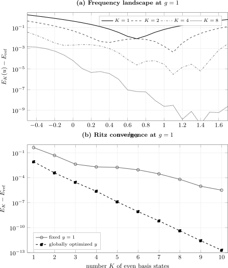
Frequency-scaled Rayleigh-Ritz results for $h=p^2/2+q^2/2+q^4$. Panel (a) shows the finite-basis energy landscape against $u=\ln y$ for $K=1,2,4,8$ even basis states. Panel (b) shows the energy excess above a $K=64$ reference. Global scale optimization accelerates finite-$K$ convergence, while the increasingly shallow multi-basin landscape makes the numerical value of the optimal scale less stable.

For $g=1$, the global minima found by the scan are:

$K$	Detected Basins	$y_K^\star$	$E_K^{\mathrm{opt}}-E_{\mathrm{ref}}$
$1$	$1$	$2.000000$	$8.72935\times10^{-3}$
$2$	$2$	$2.965439$	$4.04166\times10^{-4}$
$4$	$4$	$3.051330$	$2.50828\times10^{-6}$
$6$	$6$	$4.048019$	$8.78926\times10^{-9}$
$8$	$8$	$4.048701$	$4.37155\times10^{-11}$

The observed basin count in this finite sweep is a diagnostic, not a general theorem. Its practical message is simpler: a one-shot local search is not a reproducible global optimizer.

Coupling Sweep

The same protocol was run at weak, intermediate, and strong coupling. The reference uses $K=64$ at the analytic one-Gaussian frequency $y_{\mathrm G}$. Increasing the reference dimension from $K=32$ through $48$, $64$, and $80$ leaves all displayed reference digits unchanged.

$g$	$E_{\mathrm{ref}}$	Optimized $K=1$ Excess	Optimized $K=4$ Excess	Optimized $K=8$ Excess	Fixed-$y=1$, $K=8$ Excess
$0.1$	$0.559146327184$	$1.16104\times10^{-3}$	$1.09425\times10^{-7}$	$7.45\times10^{-13}$	$5.25918\times10^{-9}$
$1$	$0.803770651234$	$8.72935\times10^{-3}$	$2.50828\times10^{-6}$	$4.37155\times10^{-11}$	$6.69763\times10^{-5}$
$10$	$1.504972407779$	$2.62776\times10^{-2}$	$9.78734\times10^{-6}$	$2.12461\times10^{-10}$	$5.99230\times10^{-3}$

Several conclusions are visible.

Optimization matters most before convergence

At $g=10$, the unscaled $K=8$ basis is still high by about $6\times10^{-3}$, while scale optimization reduces the excess below $3\times10^{-10}$. The fixed basis is not incorrect; it is poorly matched to a much narrower wavefunction.

Shape flexibility matters beyond one Gaussian

The $K=1$ result is already a useful upper bound and has the correct strong-coupling power law. Its remaining error reflects non-Gaussian shape information. Adding even excited basis functions supplies that information while retaining parity exactly.

Tiny energy error does not determine a unique scale

At larger $K$, a broad range of frequencies spans nearly the same well-converged state. The optimized $y_K^\star$ can move between nearby basins while the energy changes below the target precision. Reporting many digits of $y_K^\star$ would confuse optimizer conditioning with physics.

Stationarity and the Virial Check

Changing $u$ dilates every basis function. For a fully optimized eigenvector inside $\mathcal V_K(e^u)$, the envelope theorem gives

$$\frac{dE_K}{du} = \langle T\rangle - \frac12\langle q^2\rangle - 2g\langle q^4\rangle.$$

Define the virial residual

$$\nu_K = 2\langle T\rangle - \langle q^2\rangle - 4g\langle q^4\rangle.$$

Then

$$\frac{dE_K}{du} = \frac12\nu_K.$$

Frequency stationarity therefore enforces the quartic-oscillator virial relation within the optimized finite trial family. This is a stronger check than merely observing that the optimizer stopped: it compares the claimed stationary point with independently assembled expectation values.

For the reported minima, $|\nu_K|$ is below $7\times10^{-8}$ and is usually much smaller. The tolerance is set by the flatness of the landscape and double-precision cancellation, not by the eigensolver residual.

Curvature and Parameter Conditioning

In the one-dimensional outer problem, the local Hessian is

$$\kappa_u = \left. \frac{d^2E_K}{du^2} \right|_{u=u_K^\star}.$$

At $g=1$, a centered finite difference gives:

$K$	$\kappa_u$
$1$	$1.37503$
$2$	$3.80834\times10^{-1}$
$4$	$4.39610\times10^{-3}$
$6$	$5.43191\times10^{-5}$
$8$	$3.37371\times10^{-7}$

Near a minimum,

$$E_K(u_K^\star+\delta u) - E_K(u_K^\star) \approx \frac12\kappa_u(\delta u)^2.$$

The falling curvature explains why $y_K^\star$ becomes difficult to locate even as the energy becomes highly accurate. A small gradient is not enough to certify a well-determined parameter when the curvature is also tiny. The broader interpretation of stiff and soft variational directions is developed in Variational Parameters and Conditioning and Stability.

Validation Ledger

The program stops with an error if any required check fails.

Harmonic limit

At $g=0$, $K=1$, and $y=1$,

$$E_1 = \frac12$$

to machine precision.

One-Gaussian agreement

For every tested $g$, the $K=1$ optimizer reproduces the positive root of

$$y^3-y-6g=0$$

and the analytic Gaussian energy.

Hermiticity and parity

The assembled matrix obeys

$$\|H_K-H_K^{\mathsf T}\| < 10^{-13}.$$

An independently assembled full-basis matrix has a vanishing even-odd block to the same tolerance.

Eigensolver residual

For the normalized lowest eigenvector,

$$\rho_K = \|H_Kc_K-E_Kc_K\|$$

is below $2\times10^{-15}$ in the published sweep. This verifies the represented matrix eigenproblem, but not basis convergence by itself.

Variational ordering

The optimized values decrease with $K$ and remain above the converged reference within a $5\times10^{-12}$ roundoff allowance. Once the excess reaches roughly $10^{-13}$, only fewer digits are reported because floating-point noise can obscure the sign of a still smaller difference.

Padding independence

Increasing the operator-construction padding from six to ten oscillator levels changes the test energy by less than $2\times10^{-14}$.

Scan refinement

The scan must bracket an interior minimum. The calculation records every detected basin and compares their refined energies, rather than trusting the first stationary point found.

Downloadable Program and Data

• Download the NumPy program
• Download the benchmark CSV

Run the benchmark with:

python variational-optimization.py --output-dir variational-output

NumPy is the only required dependency for the energies, CSV files, and validation checks. If Matplotlib is installed, the program also writes a diagnostic PNG; otherwise it reports that plotting was skipped. The published vector figure is generated independently from the retained numerical data.

The source file carries the SPDX identifier MIT; the program and generated tabular data are released under the MIT License.

Reproducibility Metadata

Item	Published Run
Operating system	Windows 11, x86-64
Python	3.12.13
NumPy	2.3.5
BLAS/LAPACK	OpenBLAS 0.3.30, 64-bit integer interface
Scalar type	IEEE 754 binary64
Couplings	$g=0.1,1,10$
Optimized dimensions	$K=1,\ldots,10$ even states
Reference dimension	$K_{\mathrm{ref}}=64$ even states
Scan coordinate	$u=\ln y$
Scan interval	$[-2,4]$ for the reported couplings
Scan points	$2401$
Basin tolerance	$2\times10^{-12}$ in $u$
Operator padding	six levels above the largest retained $n$
Random seed	none; the calculation is deterministic
License	MIT

The script prints the Python and NumPy versions. A rerun intended for archival comparison should also retain np.show_config() output because different linear-algebra backends can change the final few floating-point digits.

Known Failure Modes

Assuming one broad bracket is unimodal

A golden-section or Brent-style search is reliable only when its bracket satisfies the method’s local shape assumptions. At $K>1$, different brackets can converge to different minima. Use a global scan or a genuinely global optimizer, then refine each candidate.

Treating the basis frequency as an observable

The finite-basis scale is a representation choice. Its optimum depends on $K$, the basis family, the objective, and numerical tolerance. Only predictions stable under enlargement of the trial space should receive physical interpretation.

Optimizing below the numerical floor

When $E_K(u)$ changes by less than roundoff across a broad interval, additional optimizer iterations do not add information. Curvature estimates may change sign from cancellation. Stop reporting parameter digits before this regime.

Building powers after projection

Computing $q_K^4$ from an already truncated $q_K$ corrupts boundary matrix elements. Pad first or use analytic matrix elements.

Comparing to an unconverged reference

An apparent violation of the upper bound can mean that the alleged reference is still above the optimized trial result. Converge the reference in dimension and scale before using its difference as an error estimate.

Confusing residual error with truncation error

A tiny eigenpair residual says that $H_Kc=Ec$ was solved accurately. It says nothing about the distance between $E_K$ and the infinite-dimensional energy.

Losing the symmetry sector

Including both parities is mathematically valid, but an indexing error can mix them and hide structural mistakes. Explicit parity blocks reduce cost and provide a sharp diagnostic.

Common Mistakes

• Optimizing $y$ directly with unconstrained steps that enter $y\leq0$.
• Reporting only the optimizer’s success flag, without a landscape scan or virial residual.
• Comparing energies at different $K$ without checking that each outer minimum is global.
• Keeping many digits of $y_K^\star$ after the energy landscape has become flat.
• Claiming that scale optimization removes basis error; it only reduces it within the chosen family.
• Using a fixed reference frequency at strong coupling without testing basis convergence.
• Interpreting a below-reference value at the $10^{-15}$ level as a failure of the variational theorem.

Exercises

1. Show that the $K=1$ projected matrix reproduces the analytic Gaussian Rayleigh quotient.

Solution

For the frequency-$y$ ground state,

$$\langle q^2\rangle = \frac{1}{2y}, \qquad \langle q^4\rangle = \frac{3}{4y^2}.$$

The frequency-$y$ oscillator contribution is $y/2$, and the correction to the quadratic potential is

$$\frac{1-y^2}{2} \langle q^2\rangle = \frac{1-y^2}{4y}.$$

Therefore

$$\begin{aligned} E_1(y) &= \frac{y}{2} + \frac{1-y^2}{4y} + \frac{3g}{4y^2} \\ &= \frac{y}{4} + \frac{1}{4y} + \frac{3g}{4y^2}. \end{aligned}$$

2. Prove that independently optimizing $y$ at each $K$ preserves monotone variational convergence.

Solution

Let $y_K^\star$ minimize $E_K(y)$. Since $\mathcal V_K(y)\subset\mathcal V_{K+1}(y)$ at every fixed $y$,

$$E_{K+1}(y_K^\star) \leq E_K(y_K^\star).$$

The optimized $(K+1)$-dimensional energy cannot exceed its value at $y_K^\star$, so

$$E_{K+1}^{\mathrm{opt}} \leq E_{K+1}(y_K^\star) \leq E_K^{\mathrm{opt}}.$$

Each term is also an upper bound on $E_0$ by the variational principle.

3. Derive the relation between the scale derivative and the virial residual.

Solution

Under the dilation $u\mapsto u+\delta u$, kinetic expectation values scale as $e^{\delta u}$, quadratic moments as $e^{-\delta u}$, and quartic moments as $e^{-2\delta u}$. Differentiating at fixed optimized coefficient vector gives

$$\frac{dE_K}{du} = \langle T\rangle - \frac12\langle q^2\rangle - 2g\langle q^4\rangle.$$

Twice this expression is

$$2\langle T\rangle - \langle q^2\rangle - 4g\langle q^4\rangle,$$

which is the virial residual $\nu_K$. Thus $dE_K/du=\nu_K/2$.

4. Why can forming $q^4$ after truncating $q$ give the wrong projected operator even when only low states are retained?

Solution

A matrix element of $q^4$ contains sums over intermediate oscillator states. Starting from a retained state near the upper boundary, an intermediate application of $q$ can leave the truncated space and a later application can return. Truncating $q$ first deletes that path. Building $q^4$ in a padded space and projecting afterward retains every intermediate state needed for the desired matrix elements.

5. At $g=1$, the curvature falls from about $1.38$ at $K=1$ to $3.4\times10^{-7}$ at $K=8$. If the local frequency coordinate has an uncertainty $|\delta u|=10^{-3}$, estimate the associated energy uncertainty at each dimension.

Solution

Use

$$\Delta E \approx \frac12\kappa_u(\delta u)^2.$$

At $K=1$,

$$\Delta E \approx \frac12(1.38)10^{-6} \approx 6.9\times10^{-7}.$$

At $K=8$,

$$\begin{aligned} \Delta E &\approx \frac12 \left(3.4\times10^{-7}\right) 10^{-6} \\ &\approx 1.7\times10^{-13}. \end{aligned}$$

The same uncertainty in the optimizer coordinate matters far less once the basis is converged and the landscape is flat.

6. Design an independent check that does not use oscillator-basis diagonalization.

Solution

One option is a coordinate-space finite-difference or spectral calculation on a symmetric interval. Increase the box size and grid resolution independently, impose even parity at the origin, and converge the lowest eigenvalue below the variational excess being tested. Agreement with the Ritz sequence then compares different representations and different truncation mechanisms. A shooting method with logarithmic-derivative matching provides another independent route.

Cross-Links

• Computational Notebooks
• Anharmonic Oscillator by Variational Methods
• Variational Principle
• Rayleigh-Ritz Method
• Variational Parameters
• Gaussian Variational Methods
• Common Variational Pitfalls
• Perturbation Theory Benchmarks
• Matrix Diagonalization
• Conditioning and Stability

References

• C. M. Bender and T. T. Wu, “Anharmonic oscillator,” Physical Review 184, 1231–1260, 1969.
• T. Kato, Perturbation Theory for Linear Operators, 2nd ed., Springer, 1976.
• G. H. Golub and C. F. Van Loan, Matrix Computations, 4th ed., Johns Hopkins University Press, 2013.
• J. M. Thijssen, Computational Physics, 2nd ed., Cambridge University Press, 2007.
• R. Shankar, Principles of Quantum Mechanics, 2nd ed., Springer, 1994.
• C. M. Bender and S. A. Orszag, Advanced Mathematical Methods for Scientists and Engineers, Springer, 1999.