Mott Scattering

The Mott angular factor can be computed from individual Dirac spinors, a gamma-matrix trace, or a scalar formula. This notebook compares all three, then integrates over a finite angular acceptance. It distinguishes roundoff near suppressed backscatter, quadrature error at a fixed acceptance, and the physical divergence as the forward exclusion is removed. The scattering derivation remains at Mott Scattering.

Required background. Mott Scattering fixes the external-source normalization; Free Dirac Spinors supplies the columns and spin sums. Helpful background. Validity of the Born Approximation explains why a numerically verified leading term is not an error bound for the full physical process.

Run the investigation. The program and retained results below support the stated experiment. Follow Running an Experiment for environment and output-directory guidance. The recorded evidence applies to its stated parameters and environment.

Spin sums for a fixed Coulomb source

Use $\hbar=c=1$, $\eta=(+---)$, and $V(r)=g/r$, with signed rationalized coupling $g=qQ/(4\pi)$. The source is fixed, infinitely heavy, spinless, and pointlike. Keep only the leading external-potential Born term. The incoming and outgoing momenta have magnitude $p$, energy $E=\sqrt{p^2+m^2}$, and speed $\beta=p/E$. Spinors obey $u^\dagger u=2E$ and $\bar u u=2m$.

The explicit spinor calculation evaluates

$$S=\frac12\sum_{s,s'} \left|u_{s'}^\dagger(p')u_s(p)\right|^2.$$

Independently, the trace calculation uses

$$S=\frac12\operatorname{tr} \left[(p'\!\!\!/+m)\gamma^0 (p\!\!\!/+m)\gamma^0\right].$$

Both are compared with $4E^2[1-\beta^2\sin^2(\theta/2)]$, including oblique momenta and rotated spin bases. The corresponding cross section is

$$\begin{aligned} \frac{d\sigma}{d\Omega} &=\frac{g^2}{4p^2\beta^2\sin^4(\theta/2)}\\ &\quad\times\left[1-\beta^2\sin^2(\theta/2)\right]. \end{aligned}$$

Its units are inverse energy squared. There is no target external-state normalization or recoil phase space in this fixed-source expression. Changing the sign of $g$ changes the leading amplitude’s sign but leaves this squared result unchanged.

Stable angular factors and comparison baselines

Near ultrarelativistic backscatter, subtracting two nearly equal terms in $1-\beta^2\sin^2(\theta/2)$ can lose precision. The program instead evaluates

$$f_{\rm spin} =\cos^2\frac\theta2 +\frac{m^2}{E^2}\sin^2\frac\theta2.$$

At $\theta=\pi$, the massive value is $m^2/E^2$; the exact massless value is zero. The raw trace residuals remain available, with absolute error, error scaled by $4E^2$, and relative error when the reference signal is nonzero. A tiny scaled residual does not guarantee small relative error in a suppressed signal.

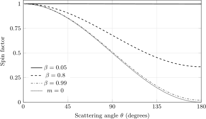
Four fixed cases from the retained angular CSV. The plotted ratio divides the matching relativistic spinless prefactor. The data start at one degree; the excluded forward cross section is not rendered finite by plotting this bounded ratio.

The spinless prefactor in this ratio is $g^2/[4p^2\beta^2\sin^4(\theta/2)]$. It is not the nonrelativistic Rutherford expression evaluated at the same mass and velocity. For the latter comparison, with $m>0$,

$$\frac{(d\sigma/d\Omega)_{\rm Mott}} {(d\sigma/d\Omega)_{\rm Rutherford,\ same\ }v} =(1-\beta^2)f_{\rm spin}.$$

The limits CSV checks this distinction as $\beta\to0$. The spin-transition CSV instead resolves the configured result in fixed Pauli seed indices. These are not momentum-helicity labels; at $m=0$ there is no rest frame. At an exactly zero spin sum, conditional transition fractions are undefined and left empty.

Finite acceptance and the forward limit

All integrated cross sections retain $0<\theta_{\min}<\theta_{\max}\le\pi$ and integrate over the full azimuth. Set $x=\sin^2(\theta/2)$. An independent closed benchmark is

$$\begin{aligned} \sigma_{\rm acc} ={}&\frac{\pi g^2}{p^2\beta^2} \Bigl[ \frac1{x_{\min}}-\frac1{x_{\max}}\\ &\qquad-\beta^2\log\frac{x_{\max}}{x_{\min}} \Bigr]. \end{aligned}$$

The numerical method applies composite Simpson quadrature in $\log x$. The independent benchmark is evaluated with 60-digit decimal arithmetic, using the supplied floating-point endpoints and value of $\pi$. This improves the evaluation of that expression; it does not turn its inputs into 60-digit data.

The fixed refinement study uses $m=1$, $p=4/3$, $|g|=0.001$ and acceptance $1^\circ\le\theta\le160^\circ$. At 256 intervals, its relative error is about $1.03\times10^{-8}$, and the last observed order is 3.99930. The custom default acceptance instead ends at $180^\circ$ and uses 2,048 intervals. Keep these rows separate when reading the convergence table.

Reducing $\theta_{\min}$ changes the physical acceptance. At fixed parameters,

$$\theta_{\min}^2\sigma_{\rm acc} \longrightarrow\frac{4\pi g^2}{p^2\beta^2} \qquad(\theta_{\min}\to0).$$

Here $\theta_{\min}$ is in radians. The cutoff CSV takes degree-valued input angles but converts them before forming this scaled quantity. The unscreened total cross section diverges. Increasing quadrature resolution cannot make that physical limit finite.

The report also records $|g|/\beta$ as a perturbative-regime diagnostic. It is not a uniform bound on omitted Coulomb terms. Screening, source size, recoil, exact Coulomb phases, radiation, loop corrections, and pair creation are outside the model. Numerical agreement among its three spin sums does not test these omitted effects.

Execute and reproduce

Download the standalone Python program. The retained run used Python 3.12.14 and NumPy 2.3.5 and passed 9,458 checks. The largest retained scaled check error comes from the finite-acceptance quadrature, so it should not be confused with the much smaller spin-algebra residuals.

python -m pip install numpy==2.3.5
python mott-scattering.py --output-dir mott-results

Existing outputs are protected. The default configured case has $m=1$, $p=4/3$, $g=-0.001$, azimuth $37^\circ$, and 181 polar angles from $1^\circ$ to $180^\circ$. Fixed reference cases run alongside it. To inspect exact massless backscatter:

python mott-scattering.py --mass 0 --momentum 1 --output-dir mott-massless

Download	Contents
Angular CSV	Spinor, trace, scalar results, two comparison baselines, and error scales
Spin transitions CSV	Configured-case Pauli seed transitions and defined conditional fractions
Limits CSV	Low-speed and high-energy comparisons with stated kinematic matching
Angular convergence CSV	Quadrature refinement at fixed acceptance and the separate configured integral
Forward cutoffs CSV	Changing physical acceptance and its scaled divergent limit
JSON report	Checks, parameters, approximation scope, environment, and hashes

The public JSON replaces local output locations with download paths; numerical results and CSV bytes retain the executed run’s values. For the figure, put the default angular CSV beside the TikZ source and use PGFPlots 1.18:

latex notebook-mott-spin-factor.tex
dvisvgm --no-fonts notebook-mott-spin-factor.dvi

The source selects four of the default 181-row blocks. Update the selection if changing the sample count.

Exercises

Two independent limits. Compare doubling the quadrature intervals at fixed acceptance with halving the lower angular cutoff. Which operation tests numerical convergence?

Solution

Only the first keeps the integral fixed. Its error approaches the independent closed value at fourth order until roundoff becomes relevant. Halving a small physical cutoff makes the leading cross section grow by about four. That is the Coulomb forward divergence, not failed quadrature convergence.

An ambiguous Rutherford ratio. At $\beta=0.8$ and $\theta=90^\circ$, compute the spin factor and the ratio to Rutherford at the same mass and velocity.

Solution

The spin factor is $1-0.64/2=0.68$. The same-velocity Rutherford ratio is $(1-0.64)\times0.68=0.2448$. The difference comes from the relativistic relation $p=E\beta$ in the prefactor, not from another spin effect.

A suppressed signal. Explain why an absolute trace error of order $10^{-15}E^2$ can be significant relative to the massive backscattering result when $E/m$ is large.

Solution

The backscattering spin sum is $4m^2$, although individual trace contributions can be of order $E^2$. The relative error can therefore grow like $(E/m)^2$ times an error scaled by $E^2$. Inspect the exported absolute and relative errors and compare with the stable scalar factor.

References

• Bjorken, James D., and Sidney D. Drell. Relativistic Quantum Mechanics. McGraw–Hill, 1964.
• DeGrand, Thomas. A One-Semester Course on Quantum Field Theory. University of Colorado lecture notes, 30 December 2025, section 8.7. Lecture text.
• Greiner, Walter. Relativistic Quantum Mechanics: Wave Equations. 3rd edition. Springer, 2000. doi:10.1007/978-3-662-04275-5.