Time-Dependent Two-Level Systems Notebook

A unitary time step can conserve probability perfectly and still produce the wrong dynamics. Exact exponentiation of a Hamiltonian frozen at each time step removes one source of error, but it does not remove time-ordering error, rotating-wave error, two-state projection error, pulse-model error, or disagreement between a closed-system model and an experiment.

This notebook turns that hierarchy into an executable benchmark. It computes:

1. resonant and detuned Rabi oscillations;
2. a full laboratory-frame evolution and its rotating-wave approximation (RWA);
3. square and Gaussian pulses with the same nominal area;
4. ideal and finite-pulse Ramsey sequences; and
5. convergence, norm, and analytic-reference diagnostics for every layer.

The retained headline results are:

Diagnostic	Computed value	Interpretation
largest matrix-versus-analytic Rabi error	$2.22\times10^{-16}$	constant-pulse implementation check
largest medium-versus-fine laboratory-frame difference	$4.65\times10^{-6}$	resolved propagation error estimate
largest lab-versus-RWA difference at $\Omega/\omega_0=0.02$	$5.04\times10^{-3}$	approximation error is resolved numerically
largest lab-versus-RWA difference at $\Omega/\omega_0=0.30$	$7.87\times10^{-2}$	weak-drive approximation degrades
resonant Gaussian area-law error	$7.31\times10^{-8}$	envelope propagation check
largest detuned square-versus-Gaussian difference	$0.2592$	equal area does not fix a detuned unitary
largest finite-versus-instantaneous Ramsey difference	$0.1915$	finite pulses alter the fringe envelope
largest retained norm error	$1.65\times10^{-13}$	propagation remains unitary to roundoff

The first two rows test different questions. The small norm error says that the numerical evolution stays on the state sphere. The convergence difference estimates how accurately the time-ordered evolution is resolved. Neither quantity says that the RWA or the two-state model is physically accurate.

Run the investigation. The program and retained results below support the stated experiment. Follow Running an Experiment for environment and output-directory guidance. The recorded evidence applies to its stated parameters and environment.

Purpose and Canonical Scope

This page is the canonical home for the executable calculation that:

• implements exact $2\times2$ exponentials for constant two-level Hamiltonians;
• checks the detuned Rabi formula against matrix propagation;
• propagates the explicitly oscillating laboratory-frame Hamiltonian with a unitary exponential-midpoint method;
• separates time-step error from laboratory-frame versus RWA discrepancy;
• verifies the resonant pulse-area theorem for square and Gaussian envelopes;
• demonstrates pulse-shape dependence away from resonance;
• constructs ideal and finite-pulse Ramsey fringes;
• generates a phase-stepped Ramsey error signal; and
• exports data, metadata, and validation thresholds in machine-readable form.

The neighboring pages retain broader canonical responsibilities:

• Two-Level Atom owns the projection from a multilevel atom, matrix-element calibration, drive phase, and detuning conventions.
• Rabi Oscillations owns the AMO interpretation of population traces, pulse calibration, Rabi chevrons, readout contrast, and experimental failure signatures.
• Rabi Oscillations: First Encounter owns the introductory closed-form solution.
• Rotating-Wave Approximation owns the approximation’s derivation, scale hierarchy, counter-rotating terms, and analytic error estimates.
• Rotating Frames owns exact time-dependent frame transformations.
• Ramsey Interferometry owns separated-field measurement physics, finite-pulse spectroscopy, frequency-discriminator design, clock noise, and systematic shifts.
• Optical Bloch Equations owns the AMO treatment of relaxation, dephasing, saturation, and fluorescence.
• ODE Solvers and Convergence Tests own the general numerical analysis.

This notebook uses those results as validation standards. It does not duplicate their full derivations, and it does not treat a generic dimensionless calculation as a species-specific prediction.

Reproducibility Contract

The executable artifact is a NumPy-only Python program:

• Download the program
• Detuned Rabi traces
• Laboratory-frame and RWA traces
• Pulse-area scan
• Ramsey scan
• Time-step convergence table
• Machine-readable metadata and validation

Run the downloaded program from the folder where you saved it:

python time-dependent-two-level.py --output-dir results

The default run declares:

Item	Choice
language	Python 3
numerical dependency	NumPy
random numbers	none
internal convention	$\hbar=1$
frequency unit	arbitrary angular-frequency unit
time unit	reciprocal angular-frequency unit
Rabi samples	$401$
laboratory-frame samples	$401$
fine carrier steps per cycle	$1600$
pulse-area samples	$161$
Gaussian midpoint steps	$1200$
Ramsey samples	$401$
matrix exponential	analytic Pauli-matrix formula
time-dependent integrator	exponential midpoint

The program has no fitted correction, stochastic seed, hidden optimizer, external solver, or plotting dependency. The CSV files contain the data used by the figure, while the JSON record preserves conventions, parameters, runtime versions, acceptance checks, provenance identifiers, and limitations.

Claim boundary

The calculation is a closed-system propagator and approximation benchmark. It assumes that a two-state projection has already been justified. It does not include:

• spontaneous emission or population relaxation;
• pure dephasing;
• leakage to spectator levels;
• atomic motion or Doppler averaging;
• spatial intensity inhomogeneity;
• pulse-generator transfer functions;
• state-preparation and measurement errors; or
• uncertainty in species-specific transition parameters.

Those omissions are not small-print details. For a real experiment, they can dominate a numerically converged two-state trajectory.

Conventions Before Code

Two-level calculations are unusually vulnerable to silent sign and factor-of-two errors. The implementation therefore fixes its conventions before any propagation.

The ordered basis is

$$\begin{pmatrix} |e\rangle\\ |g\rangle \end{pmatrix},$$

represented by

$$|e\rangle= \begin{pmatrix} 1\\0 \end{pmatrix}, \qquad |g\rangle= \begin{pmatrix} 0\\1 \end{pmatrix}.$$

The Pauli matrices are

$$\sigma_x= \begin{pmatrix} 0&1\\ 1&0 \end{pmatrix}, \qquad \sigma_y= \begin{pmatrix} 0&-i\\ i&0 \end{pmatrix},$$

and

$$\sigma_z= \begin{pmatrix} 1&0\\ 0&-1 \end{pmatrix}.$$

Thus $|e\rangle$ and $|g\rangle$ have $\sigma_z$ eigenvalues $+1$ and $-1$, respectively. The detuning is

$$\Delta=\omega_0-\omega_L.$$

A positive detuning therefore means that the unperturbed transition frequency lies above the drive frequency. Some texts use the opposite sign. Population curves with phase zero can hide this difference because they are often even in $\Delta$, while coherences and phase-stepped Ramsey signals cannot.

The phase-dependent transverse operator is

$$\sigma_\phi = \cos\phi\,\sigma_x + \sin\phi\,\sigma_y.$$

The RWA Hamiltonian used by every constant pulse is

$$\frac{H_{\mathrm{RWA}}}{\hbar} = \frac12 \left( \Delta\sigma_z+\Omega\sigma_\phi \right).$$

The corresponding laboratory-frame Hamiltonian is

$$\frac{H_{\mathrm{lab}}(t)}{\hbar} = \frac{\omega_0}{2}\sigma_z + \Omega \cos(\omega_Lt+\phi)\sigma_x.$$

With this linear-drive convention, the near-resonant co-rotating term produces the same $\Omega$ that appears in the RWA Hamiltonian. Replacing the laboratory coupling by $2\Omega\cos(\omega_Lt)\sigma_x$ would double the RWA coupling and invalidate the comparison.

Exact Propagators for Constant Segments

Any traceless Hermitian two-state Hamiltonian can be written

$$\frac{H}{\hbar} = h_x\sigma_x+h_y\sigma_y+h_z\sigma_z.$$

Define

$$h = \sqrt{h_x^2+h_y^2+h_z^2}.$$

Because

$$\left( h_x\sigma_x+h_y\sigma_y+h_z\sigma_z \right)^2 = h^2I,$$

its propagator is

$$\begin{aligned} U(\delta t) &= \exp\left( -iH\delta t/\hbar \right) \\ &= \cos(h\delta t)I - i\frac{\sin(h\delta t)}{h} \left( h_x\sigma_x+h_y\sigma_y+h_z\sigma_z \right). \end{aligned}$$

The code evaluates this expression directly. For $h=0$, it returns the identity rather than dividing by zero.

This formula has three practical advantages:

1. every constant segment is unitary up to floating-point roundoff;
2. no generic matrix-exponential dependency is required; and
3. the factor-of-two convention is visible in the coefficients.

It does not solve an arbitrary time-dependent problem exactly. When $H(t_1)$ and $H(t_2)$ do not commute, a product of frozen-Hamiltonian propagators still approximates a time-ordered exponential.

Detuned Rabi Benchmark

For a constant RWA pulse of phase zero and initial state $|g\rangle$, define

$$\Omega_R = \sqrt{\Omega^2+\Delta^2}.$$

The analytic excited-state probability is

$$P_e(t) = \frac{\Omega^2}{\Omega_R^2} \sin^2\left( \frac{\Omega_Rt}{2} \right).$$

The notebook uses $\Omega=1$ and scans

$$\frac{\Delta}{\Omega} \in \left\{ 0,\frac12,1 \right\}$$

over $0\le\Omega t\le4\pi$. It computes each point twice:

• directly from the analytic probability; and
• by applying the exact constant-segment matrix propagator to $|g\rangle$.

The largest probability difference is at floating-point scale. This test catches:

• a reversed basis;
• an omitted factor of $1/2$;
• a mistaken generalized Rabi frequency;
• an amplitude prefactor error;
• a projection onto the wrong state; and
• a nonunitary propagator implementation.

What detuning changes

Detuning changes both the oscillation rate and its amplitude:

$$\text{frequency}=\Omega_R, \qquad P_e^{\max} = \frac{\Omega^2}{\Omega^2+\Delta^2}.$$

For the three retained cases:

$\Delta/\Omega$	$\Omega_R/\Omega$	$P_e^{\max}$
$0$	$1$	$1$
$0.5$	$\sqrt{1.25}\approx1.118$	$0.8$
$1$	$\sqrt2\approx1.414$	$0.5$

The oscillations speed up while complete inversion becomes impossible. A single fitted sinusoid with an unconstrained amplitude can therefore conceal whether a reduced contrast came from detuning, dephasing, readout, leakage, or inhomogeneity.

Time-Dependent Laboratory-Frame Propagation

The full comparison retains the counter-rotating part of the linear drive:

$$\frac{H_{\mathrm{lab}}(t)}{\hbar} = \frac{\omega_0}{2}\sigma_z + \Omega\cos(\omega_Lt)\sigma_x.$$

The benchmark sets

$$\omega_0=\omega_L=1$$

and scans

$$\eta = \frac{\Omega}{\omega_0} \in \left\{ 0.02,0.05,0.10,0.20,0.30 \right\}.$$

The horizontal coordinate is the slow time

$$\tau=\Omega t,$$

so every case covers $0\le\tau\le2\pi$. As $\eta$ decreases, the same slow Rabi interval contains more carrier cycles. That is precisely the scale separation on which the RWA relies.

Exponential-midpoint update

For a step from $t_n$ to $t_{n+1}=t_n+\delta t$, the program samples the Hamiltonian at the midpoint:

$$t_{n+1/2} = t_n+\frac{\delta t}{2}.$$

It then updates

$$|\psi_{n+1}\rangle = \exp\left[ -\frac{i\delta t}{\hbar} H(t_{n+1/2}) \right] |\psi_n\rangle.$$

Each frozen exponential is evaluated with the Pauli formula. The method is time symmetric and has second-order global accuracy for a smooth Hamiltonian:

$$\left\| |\psi_{\mathrm{num}}(T)\rangle - |\psi(T)\rangle \right\| = O(\delta t^2)$$

at fixed final time, subject to regularity and stability assumptions.

The exact unitary of each substep ensures

$$\langle\psi_{n+1}|\psi_{n+1}\rangle = \langle\psi_n|\psi_n\rangle$$

in exact arithmetic. It does not ensure that the ordered product equals the exact time-ordered propagator. Norm preservation is therefore a necessary structural check, not a convergence proof.

Sampling and internal stepping are distinct

The CSV trace has $401$ requested output times. Between two output times, the integrator may take several internal steps so that no internal step exceeds

$$\delta t_{\max} = \frac{2\pi} {\omega_LN_c},$$

where $N_c$ is the requested number of steps per carrier cycle. This separation prevents plotting resolution from silently controlling solver accuracy.

The retained convergence ladder is

$$N_c=400,\ 800,\ 1600.$$

Rotating-Wave Comparison

On exact resonance, the corresponding RWA prediction is

$$P_e^{\mathrm{RWA}}(\tau) = \sin^2\left( \frac{\tau}{2} \right).$$

The notebook compares this curve with the converged laboratory-frame result at identical $\Omega$. The retained diagnostics are:

$\Omega/\omega_0$	$400$ versus $800$	$800$ versus $1600$	lab versus RWA	lab $P_e$ at nominal $\pi$ pulse
$0.02$	$1.85\times10^{-5}$	$4.65\times10^{-6}$	$5.04\times10^{-3}$	$0.9999750$
$0.05$	$1.77\times10^{-5}$	$4.57\times10^{-6}$	$1.22\times10^{-2}$	$0.9998435$
$0.10$	$1.70\times10^{-5}$	$4.52\times10^{-6}$	$2.58\times10^{-2}$	$0.9993712$
$0.20$	$1.56\times10^{-5}$	$4.35\times10^{-6}$	$5.40\times10^{-2}$	$0.9974391$
$0.30$	$1.22\times10^{-5}$	$4.43\times10^{-6}$	$7.87\times10^{-2}$	$0.9950235$

At the weakest drive, the maximum RWA discrepancy is more than one thousand times the medium-to-fine propagation difference. The mismatch is therefore resolved; reducing the time step cannot make it disappear.

Interpreting the discrepancy carefully

The reported lab-versus-RWA value is the maximum pointwise population difference over a finite interval. It combines:

• fast micromotion from the counter-rotating component;
• an accumulated phase difference;
• the leading counter-rotating frequency shift;
• changes in the effective rotation axis; and
• the chosen start phase and observation window.

It is not a universal RWA error bound. A stroboscopic comparison, a phase-averaged comparison, a gate infidelity, a quasienergy difference, and a maximum pointwise population difference answer different questions.

The systematic growth across the selected drive ratios supports the expected weak-drive hierarchy. It does not establish one exact power law from five finite-window points.

Why nominal inversion remains high

The maximum trace discrepancy reaches nearly $0.08$ at $\Omega/\omega_0=0.30$, while the population at the nominal RWA $\pi$ pulse is still about $0.995$. These statements are compatible. A pointwise maximum can occur away from the nominal gate time, and fast micromotion can be large locally while partially canceling at a selected endpoint.

For control design, the endpoint unitary or process fidelity is often more relevant than the largest transient population difference. For spectroscopy, the accumulated phase or resonance shift may matter more. The diagnostic must follow the intended observable.

Pulse Area

For a phase-fixed resonant RWA pulse with time-dependent envelope $\Omega(t)$,

$$\frac{H(t)}{\hbar} = \frac{\Omega(t)}{2}\sigma_x.$$

Hamiltonians at all times commute:

$$[H(t_1),H(t_2)]=0.$$

The propagator depends only on the pulse area

$$\Theta = \int_0^{t_p}\Omega(t)\,dt,$$

and an initial ground state has

$$P_e(t_p) = \sin^2\left( \frac{\Theta}{2} \right).$$

This is not restricted to square pulses. It holds for any integrable amplitude envelope under the stated resonant, fixed-axis, closed-system Hamiltonian.

Square pulse

For duration $t_p=1$, the square envelope is

$$\Omega_{\mathrm{sq}}(t) = \Theta.$$

The constant propagator reproduces the area law with maximum discrepancy $2.22\times10^{-16}$ over

$$0\le\Theta\le4\pi.$$

Truncated Gaussian pulse

The comparison Gaussian is centered at $t_p/2$ with width

$$\sigma=0.15t_p.$$

It is normalized on the finite pulse interval:

$$\Omega_{\mathrm G}(t) = \frac{\Theta} {\sigma\sqrt{2\pi}\, \operatorname{erf} \left[ t_p/(2\sqrt2\sigma) \right]} \exp\left[ -\frac{(t-t_p/2)^2}{2\sigma^2} \right].$$

Thus

$$\int_0^{t_p}\Omega_{\mathrm G}(t)\,dt = \Theta$$

analytically. Exponential-midpoint propagation with $1200$ steps reproduces the area law to $7.31\times10^{-8}$ in probability. That finite error is a quadrature and time-ordering discretization diagnostic, not a failure of the area theorem.

Equal area away from resonance

At detuning $\Delta=2$,

$$\frac{H(t)}{\hbar} = \frac12 \left[ \Delta\sigma_z+\Omega(t)\sigma_x \right].$$

Now

$$\begin{aligned} [H(t_1),H(t_2)] &= \frac{i\hbar^2\Delta}{2} \left[ \Omega(t_2)-\Omega(t_1) \right]\sigma_y, \end{aligned}$$

which is generally nonzero. Equal area no longer implies equal evolution. The detuning term acts during the pulse, and its noncommuting combination with the changing transverse drive remembers the envelope.

Across the retained scan, the maximum square-versus-Gaussian population difference is

$$0.2592125409.$$

At nominal area $\Theta=\pi$:

$$\begin{aligned} P_e^{\mathrm{square}} &= 0.6529052079, \\ P_e^{\mathrm{Gaussian}} &= 0.9054075396. \end{aligned}$$

The difference is not caused by unequal numerical area: both envelopes use the same declared $\Theta$. It is a physical consequence of noncommuting dynamics within the chosen model.

Ramsey Sequences

The benchmark sequence is:

$$\frac{\pi}{2}\text{ pulse} \quad\longrightarrow\quad \text{free evolution for }T \quad\longrightarrow\quad \frac{\pi}{2}\text{ pulse}.$$

The first pulse creates a coherent superposition. During the free interval, the relative phase advances with detuning. The second pulse maps that phase to population.

Instantaneous-pulse reference

For ideal resonant pulses with phases $\phi_1$ and $\phi_2$, the reference probability is

$$P_e^{\mathrm{ideal}} = \frac12 \left[ 1+ \cos\left( \Delta T+\phi_1-\phi_2 \right) \right].$$

The program also constructs the corresponding sequence from exact matrix propagators. The maximum formula-versus-matrix discrepancy over the retained grid is $5.55\times10^{-16}$.

This check is intentionally independent of the plotted finite-pulse sequence. It verifies pulse order, phase sign, basis order, and the free evolution convention.

Finite pulses

The finite sequence uses

$$\Omega_p=4, \qquad t_p = \frac{\pi}{2\Omega_p} = \frac{\pi}{8}, \qquad T=10.$$

During each pulse, the Hamiltonian includes the same detuning used during free evolution:

$$\frac{H_p}{\hbar} = \frac12 \left( \Delta\sigma_z+\Omega_p\sigma_\phi \right).$$

The pulse is therefore an exact $\pi/2$ rotation only at $\Delta=0$. Away from resonance, its axis tilts and its angle changes. Compared with the instantaneous-pulse curve, the finite-pulse fringe acquires a modified envelope and phase.

The largest population difference over

$$-1\le\Delta\le1$$

is $0.1915320568$. This is a model difference, not numerical noise: every segment has an exact constant Hamiltonian.

On-resonance checks

For zero relative pulse phase at $\Delta=0$, the two $\pi/2$ pulses combine to a $\pi$ rotation:

$$P_e(0)=1.$$

With the second pulse shifted by $\pm\pi/2$, the on-resonance populations are

$$P_e^{(+)}(0) = P_e^{(-)}(0) = \frac12.$$

These values test both pulse calibration and the implementation of $\sigma_\phi$.

Phase-stepped error signal

Define

$$\mathcal E(\Delta) = P_e^{(+\pi/2)}(\Delta) - P_e^{(-\pi/2)}(\Delta).$$

The error signal crosses zero on resonance:

$$\mathcal E(0)=0.$$

A centered finite difference on the exported grid gives

$$\left. \frac{d\mathcal E}{d\Delta} \right|_{\Delta=0} = 10.49517719.$$

For instantaneous pulses in this convention, the magnitude of the corresponding central slope is $T=10$. The finite-pulse value is larger because phase also accumulates during the two pulses. Treating the dark time as the entire interrogation time would miss that contribution.

The sign of an experimental discriminator depends on the detuning and phase-step conventions. Its zero crossing and calibrated slope are more robust records than a bare statement that the signal is “dispersive.”

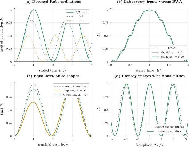
Four closed-system checks generated from the downloadable CSV files. Panel (a) verifies the detuned Rabi frequency and amplitude. Panel (b) resolves carrier-scale micromotion and accumulated RWA discrepancy at weak and moderate drive. Panel (c) shows that resonant evolution depends only on pulse area, whereas equal-area square and Gaussian pulses differ at $\Delta=2$. Panel (d) compares instantaneous and finite $\pi/2$ Ramsey pulses. Curves are dimensionless model results, not a fit to a particular atom.

What the Figure Does Not Show

A compact figure necessarily suppresses several diagnostics that remain in the data:

• panel (a) exports both analytic and matrix-propagated columns for every detuning;
• panel (b) exports all five drive ratios, not only the two displayed;
• the convergence CSV contains coarse, medium, and fine differences for each laboratory trace;
• panel (c) exports square and Gaussian results on and off resonance;
• panel (d) exports both $\pm\pi/2$ phase steps and their difference;
• the metadata records the maximum norm error for each calculation; and
• validation thresholds are machine-readable rather than inferred from plot thickness.

A plot is an interface to the calculation, not its complete evidentiary record.

Validation Architecture

The notebook uses a ladder of checks rather than one omnibus comparison.

Level 1: algebra

The Pauli matrices obey

$$\sigma_i^2=I$$

and the propagator formula follows from that identity. Constant RWA segments are compared with known analytic probabilities.

Level 2: structure

Every propagator is unitary in exact arithmetic. The largest retained norm error is

$$1.65\times10^{-13}.$$

This catches implementation failures such as a sign error in the imaginary exponential coefficient or accidental use of a non-Hermitian Hamiltonian.

Level 3: time-step convergence

The full laboratory-frame problem is recomputed at $400$, $800$, and $1600$ steps per carrier cycle. The fine-level difference is compared with the physical RWA discrepancy.

For a second-order method, halving the step should reduce an asymptotic error by about four. The coarse-to-medium differences are roughly four times the medium-to-fine differences, consistent with the expected regime:

$$\frac{ \|P_{400}-P_{800}\|_\infty }{ \|P_{800}-P_{1600}\|_\infty } \approx 3\text{ to }4.$$

The ratio is not exactly four because the diagnostic is a maximum over a sampled trajectory, floating-point effects are present, and the maximizing time can change with resolution.

Level 4: approximation separation

The acceptance check requires the weak-drive RWA discrepancy to exceed the weak-drive medium-to-fine numerical difference by more than a factor of $500$. The actual ratio is about

$$\frac{5.04\times10^{-3}} {4.65\times10^{-6}} \approx1084.$$

This prevents a calculation from declaring an approximation failure when it has not first resolved the reference dynamics.

Level 5: physical identities

Independent identities test different workflows:

• detuned Rabi formula;
• resonant area theorem;
• ideal Ramsey formula;
• resonant two-pulse inversion;
• zero crossing of the phase-stepped error signal.

Agreement among these tests is stronger than agreement with one curve generated by the same code path.

Error Ledger

For a species-specific driven transition, a useful hierarchy is:

Layer	Question	Representative diagnostic
Hilbert-space projection	Are two states isolated?	spectator detunings, leakage calculation
Hamiltonian calibration	Are $\omega_0$, $\Omega$, $\phi$, and polarization correct?	independent spectroscopy and power calibration
frame choice	Are observables transformed consistently?	exact rotating-frame identity
approximation	Is the RWA adequate?	lab-frame comparison or controlled expansion
pulse model	Does the delivered field match the envelope?	measured transfer function and waveform
propagation	Is time ordering resolved?	step-size convergence
floating point	Is unitarity retained?	norm and reversibility checks
open-system model	Are $T_1$, $T_2$, and noise included?	master-equation comparison
ensemble model	Are motion and inhomogeneity included?	distribution average
readout	Does computed population map to counts?	calibrated measurement model

The present notebook addresses the frame, approximation, pulse-model, and propagation rows within an idealized two-state closed system. It does not collapse the remaining rows into a single numerical error bar.

Projection error

A real atom has additional Zeeman, hyperfine, fine-structure, motional, and possibly continuum states. Even if none is appreciably populated, virtual couplings can shift the two-state resonance. The ratio $\Omega/\omega_0$ used in the lab-versus-RWA benchmark says nothing by itself about $\Omega$ relative to the nearest spectator-state detuning.

Approximation error

The RWA removes counter-rotating terms after a frame transformation. Its validity depends on drive strength, detuning, duration, phase, and target observable. A small instantaneous population error does not guarantee a small phase error after many cycles.

Propagation error

The exponential-midpoint method is exactly unitary per step, but it approximates time ordering. The relevant check is convergence of the target observable, state, or unitary, not only the norm.

Model-to-experiment error

Relaxation, phase noise, amplitude noise, finite temperature, Doppler shifts, and readout errors can reshape a Rabi or Ramsey trace. Fitting such a trace with a closed-system curve may return precise but biased parameters.

Reading the Exported Data

Detuned Rabi CSV

The columns include:

• tau and tau_over_pi;
• an analytic population for each detuning ratio; and
• a matrix-propagated population for the same ratio.

Keeping both columns makes the validation reproducible without rerunning Python.

Laboratory-frame CSV

The columns include:

• slow time $\tau=\Omega t$;
• the resonant RWA population; and
• one fine-grid laboratory-frame population for every $\Omega/\omega_0$.

The physical time differs among drive ratios because each trace uses the same slow interval.

Convergence CSV

Each row records:

• drive ratio;
• all three carrier-step counts;
• maximum coarse-to-medium difference;
• maximum medium-to-fine difference;
• maximum fine-lab-to-RWA difference;
• nominal $\pi$-pulse populations; and
• fine-grid norm error.

This table should accompany any claim based on panel (b).

Pulse-area CSV

For each area, the file contains:

• analytic area-law probability;
• resonant square result;
• resonant Gaussian result;
• detuned square result; and
• detuned Gaussian result.

The file supports direct checks of both the theorem and its failure outside the commuting regime.

Ramsey CSV

For each detuning, the file contains:

• $\Delta/\Omega_p$;
• free phase $\Delta T/\pi$;
• ideal formula and ideal matrix results;
• finite-pulse zero-phase population;
• finite-pulse $\pm\pi/2$ populations; and
• their difference as an error signal.

Reporting $\Delta T/\pi$ and $\Delta/\Omega_p$ exposes the two independent scales governing dark evolution and pulse distortion.

Extending the Calculation

Compare full unitaries

Population from one initial state does not determine a quantum operation. For gate assessment, propagate both basis vectors and assemble

$$U_{\mathrm{num}} = \begin{pmatrix} U|e\rangle & U|g\rangle \end{pmatrix}.$$

Remove an irrelevant global phase before comparing with a target unitary. Useful metrics include operator norm, average gate fidelity, worst-case state fidelity, and phase error. Declare which one is used.

Add adaptive stepping

An embedded commutator-free or Runge–Kutta method can adapt to a shaped pulse. The tolerance must be validated against a tighter run, and any nonunitary intermediate method should track norm drift separately from local error.

Add a Magnus or Floquet benchmark

For periodic driving, one can compare:

• direct laboratory propagation;
• a truncated Magnus effective Hamiltonian;
• a Floquet quasienergy calculation; and
• the leading RWA.

Quasienergies require a declared Brillouin-zone convention, while micromotion requires more than a stroboscopic effective Hamiltonian. See Floquet Theory and Magnus Expansion.

Add arbitrary envelopes

Replace the built-in square or Gaussian with sampled in-phase and quadrature controls:

$$\frac{H(t)}{\hbar} = \frac{\Delta}{2}\sigma_z + \frac{\Omega_x(t)}{2}\sigma_x + \frac{\Omega_y(t)}{2}\sigma_y.$$

Preserve:

• waveform sampling rate;
• interpolation rule;
• amplitude and phase units;
• truncation window;
• transfer-function correction;
• time origin; and
• any filter or resampling operation.

An “arbitrary waveform” without those records is not reproducible.

Add relaxation and dephasing

A density-matrix extension can use

$$\dot\rho = -\frac{i}{\hbar}[H,\rho] + \gamma_1\mathcal D[\sigma_-]\rho + \frac{\gamma_\phi}{2} \mathcal D[\sigma_z]\rho,$$

where

$$\mathcal D[L]\rho = L\rho L^\dagger - \frac12 \left\{ L^\dagger L,\rho \right\}.$$

That extension should validate:

• trace preservation;
• Hermiticity;
• positivity;
• the no-drive relaxation law;
• the resonant steady state; and
• recovery of this unitary notebook when rates vanish.

The Optical Bloch Equation Notebook owns that next computational layer.

Add leakage

Enlarge the Hamiltonian to include a spectator state. Compare:

• final target-state population;
• total leakage;
• ac Stark shift;
• effective two-state model;
• pulse-shape sensitivity; and
• convergence with respect to included states.

This separates failure of the two-state projection from failure of the RWA inside the projected subspace.

Add ensemble averaging

For a distribution $f(\Delta,\Omega)$, an incoherent measurement average is

$$\overline{P_e}(t) = \int d\Delta\,d\Omega\, f(\Delta,\Omega) P_e(t;\Delta,\Omega).$$

Average probabilities only when ensemble members are incoherent. If amplitudes interfere before detection, the averaging must occur at the state or field level.

Add optimal control

Control optimization should keep the forward propagator, objective, gradient, constraints, robustness ensemble, and final independent validation distinct. An optimizer can exploit discretization artifacts unless the optimized pulse is re-evaluated on a finer grid and, where relevant, in the full laboratory-frame or multilevel model.

Common Mistakes

Hiding the detuning sign

The population of a single zero-phase pulse can be even in $\Delta$. Coherence phases and Ramsey error signals are not. State the sign convention at the top of the calculation.

Losing a factor of two

The coefficients in

$$H_{\mathrm{RWA}} = \frac{\hbar}{2} \left( \Delta\sigma_z+\Omega\sigma_x \right)$$

imply a resonant $\pi$-pulse time $t_\pi=\pi/\Omega$. A different laboratory-drive convention changes that mapping.

Calling norm preservation convergence

A product of inaccurate unitary steps remains unitary. Repeat the target observable at smaller steps.

Comparing unresolved dynamics with an approximation

If the lab-versus-RWA discrepancy is comparable to the numerical coarse-versus-fine difference, the reference trajectory is not adequate to measure approximation error.

Using output samples as solver steps

A smooth plot can be generated from a poorly resolved propagator, while an accurate propagator can be sampled sparsely. Record both grids.

Treating maximum pointwise error as universal

The maximum depends on interval, phase, observable, and sampling. Gate infidelity, quasienergy error, and transient population error are different metrics.

Assuming equal area means equal pulse

The area theorem requires a fixed commuting rotation axis. Detuning, phase chirp, quadrature modulation, and additional levels generally break that condition.

Omitting detuning during finite pulses

Turning off $\Delta$ in a simulated Ramsey pulse while retaining it during the dark time creates the instantaneous-pulse approximation, even if the pulse has a nonzero duration in code.

Comparing only the central Ramsey fringe

Finite pulses can preserve the on-resonance value while changing side fringes, slope, and envelope. Scan a range wide enough to expose those changes.

Inferring decoherence from one damped trace

Detuning distributions, amplitude inhomogeneity, leakage, motion, technical noise, and readout can all reduce contrast. A phenomenological exponential fit is not by itself a microscopic diagnosis.

Reporting arbitrary units as a species prediction

Dimensionless results become physical only after a documented mapping of $\omega_0$, $\Omega$, time, polarization, and matrix elements to a particular transition.

Dropping metadata after plotting

CSV curves without conventions, parameters, and validation thresholds are ambiguous. Keep the machine-readable record with the figure.

Exercises

Exercise 1: exact Pauli exponential

Let

$$A=\mathbf h\cdot\boldsymbol\sigma.$$

Show that $A^2=h^2I$ and derive the exact propagator used by the notebook. Explain why the formula is continuous as $h\to0$.

Solution

The Pauli product identity is

$$\sigma_i\sigma_j = \delta_{ij}I + i\sum_k\epsilon_{ijk}\sigma_k.$$

Therefore

$$\begin{aligned} A^2 &= \sum_{ij}h_ih_j\sigma_i\sigma_j \\ &= \sum_i h_i^2I + i\sum_{ijk} h_ih_j\epsilon_{ijk}\sigma_k. \end{aligned}$$

The second term vanishes because $h_ih_j$ is symmetric in $i,j$, whereas $\epsilon_{ijk}$ is antisymmetric. Hence

$$A^2=h^2I.$$

Separate the exponential series into even and odd powers:

$$\begin{aligned} e^{-iA t} &= \sum_{n=0}^{\infty} \frac{(-1)^n(A t)^{2n}}{(2n)!} - i \sum_{n=0}^{\infty} \frac{(-1)^n(A t)^{2n+1}}{(2n+1)!} \\ &= \cos(ht)I - i\frac{\sin(ht)}{h}A. \end{aligned}$$

As $h\to0$,

$$\frac{\sin(ht)}{h}\to t,$$

while $A\to0$. Thus the expression tends continuously to $I$. The code handles $h=0$ explicitly to avoid a numerical division by zero.

Exercise 2: detuned Rabi ceiling

For fixed $\Omega$, find the first time at which the detuned Rabi probability reaches its maximum. Evaluate the maximum and time for $\Delta/\Omega=1$.

Solution

The probability is

$$P_e(t) = \frac{\Omega^2}{\Omega_R^2} \sin^2\left( \frac{\Omega_Rt}{2} \right), \qquad \Omega_R=\sqrt{\Omega^2+\Delta^2}.$$

The first maximum of the sine squared occurs when

$$\frac{\Omega_Rt}{2} = \frac{\pi}{2},$$

so

$$t_{\max} = \frac{\pi}{\Omega_R}.$$

For $\Delta=\Omega$,

$$\Omega_R=\sqrt2\,\Omega,$$

and therefore

$$t_{\max} = \frac{\pi}{\sqrt2\,\Omega}, \qquad P_e^{\max} = \frac{\Omega^2}{2\Omega^2} = \frac12.$$

The maximum arrives earlier than the resonant $\pi$ pulse, but it does not invert the population.

Exercise 3: norm versus accuracy

Construct a simple example showing that a unitary numerical propagator can have arbitrarily large phase error while preserving norm exactly.

Solution

Consider the exact Hamiltonian

$$H = \frac{\hbar\omega}{2}\sigma_z$$

and an inaccurate numerical model

$$\widetilde H = \frac{\hbar(\omega+\epsilon)}{2}\sigma_z.$$

Both propagators,

$$U(t) = e^{-i\omega t\sigma_z/2}, \qquad \widetilde U(t) = e^{-i(\omega+\epsilon)t\sigma_z/2},$$

are exactly unitary, so every state retains norm one under either evolution. For a superposition, however, the relative phase error is

$$\delta\varphi=\epsilon t.$$

At $t=\pi/|\epsilon|$, the relative phase is wrong by $\pi$, which can make an interference probability maximally wrong. Norm preservation detects no problem. Convergence or comparison of the phase-sensitive observable is required.

Exercise 4: midpoint convergence ratio

Suppose the leading population error of the laboratory propagator is

$$P_h(t)-P(t)=C(t)h^2+O(h^4).$$

Show why the difference between runs at $h$ and $h/2$ should be about four times the difference between runs at $h/2$ and $h/4$.

Solution

At a fixed time,

$$\begin{aligned} P_h-P_{h/2} &= C h^2 - C\frac{h^2}{4} + O(h^4) \\ &= \frac34Ch^2+O(h^4). \end{aligned}$$

Similarly,

$$\begin{aligned} P_{h/2}-P_{h/4} &= C\frac{h^2}{4} - C\frac{h^2}{16} + O(h^4) \\ &= \frac{3}{16}Ch^2+O(h^4). \end{aligned}$$

The leading ratio is therefore

$$\frac{|P_h-P_{h/2}|} {|P_{h/2}-P_{h/4}|} \to4.$$

For a maximum over time, the observed ratio need not be exactly four because the maximizing time may differ among resolutions. A ratio near four across several refinements is evidence for, not a proof of, the asymptotic second-order regime.

Exercise 5: resonant area theorem

Prove that any two real, fixed-phase resonant envelopes with the same area produce the same final propagator in the two-level RWA model. Identify three ways the conclusion can fail.

Solution

At resonance and fixed phase zero,

$$H(t) = \frac{\hbar\Omega(t)}{2}\sigma_x.$$

Every Hamiltonian is proportional to the same matrix, so

$$[H(t_1),H(t_2)]=0.$$

Time ordering is unnecessary:

$$\begin{aligned} U(t_p) &= \exp\left[ -\frac{i}{\hbar} \int_0^{t_p}H(t)\,dt \right] \\ &= \exp\left( -\frac{i\Theta}{2}\sigma_x \right). \end{aligned}$$

Thus the final propagator depends only on

$$\Theta=\int_0^{t_p}\Omega(t)\,dt.$$

The conclusion can fail if:

• $\Delta\ne0$, introducing a noncommuting $\sigma_z$ term;
• the drive phase varies, changing the transverse rotation axis;
• additional levels participate, so the same scalar envelope multiplies several unequal transitions;
• relaxation or dephasing acts during envelopes of different duration; or
• the laboratory-frame counter-rotating term is retained outside the RWA.

Any three of these provide the requested failure mechanisms.

Exercise 6: detuned square pulse

For a square pulse of duration $t_p=1$, area $\Theta=\pi$, and detuning $\Delta=2$, use the constant-pulse formula to reproduce the notebook’s square-pulse population.

Solution

The square amplitude is

$$\Omega=\frac{\Theta}{t_p}=\pi.$$

The generalized Rabi frequency is

$$\Omega_R = \sqrt{\pi^2+4}.$$

The final population is

$$\begin{aligned} P_e &= \frac{\pi^2}{\pi^2+4} \sin^2\left( \frac{\sqrt{\pi^2+4}}{2} \right) \\ &\approx 0.6529052079. \end{aligned}$$

This agrees with the exported square-pulse value. The resonant area-law prediction would be $1$, showing that nominal area alone is insufficient when $\Delta\ne0$.

Exercise 7: ideal Ramsey phase

Starting from $|g\rangle$, use the notebook’s pulse convention to derive

$$P_e = \frac12 \left[ 1+\cos(\Delta T+\phi_1-\phi_2) \right].$$

What happens if the detuning convention is reversed?

Solution

A resonant $\pi/2$ pulse of phase $\phi$ is

$$U_{\pi/2}(\phi) = \frac{1}{\sqrt2} \left( I-i\sigma_\phi \right).$$

Free evolution is

$$U_f = \exp\left( -\frac{i\Delta T}{2}\sigma_z \right).$$

Applying

$$U_{\pi/2}(\phi_2) U_f U_{\pi/2}(\phi_1)$$

to $|g\rangle$ and projecting onto $|e\rangle$ gives an amplitude whose modulus squared is

$$P_e = \frac12 \left[ 1+\cos(\Delta T+\phi_1-\phi_2) \right].$$

If detuning is instead defined as

$$\Delta'=\omega_L-\omega_0=-\Delta,$$

the phase becomes

$$-\Delta'T+\phi_1-\phi_2.$$

For zero pulse-phase difference, the cosine population is unchanged. For a phase-stepped error signal, the slope changes sign. That is why the detuning convention cannot be inferred safely from an unshifted Ramsey fringe alone.

Exercise 8: finite-pulse effective time

The ideal error-signal slope has magnitude $T=10$, while the finite-pulse calculation gives approximately $10.495$. Give a physical interpretation and compare the excess with the total pulse duration.

Solution

The two finite pulses each last

$$t_p=\frac{\pi}{8}\approx0.392699.$$

Their total duration is

$$2t_p\approx0.785398.$$

Detuning acts during the pulses as well as during the free interval. The phase-to-population sensitivity therefore corresponds to an effective interrogation time larger than $T$. The observed excess is

$$10.495177-10 \approx0.495177.$$

This is smaller than the full pulse duration because a driven state does not accumulate Ramsey phase during a pulse in the same way as during free precession. The rotating axis and changing population weight the detuning response.

The result should not be summarized by simply replacing $T$ with $T+2t_p$. The exact effective sensitivity follows from the finite-pulse propagator or a sensitivity-function calculation.

Exercise 9: design a stronger RWA test

The notebook compares one initial state through a maximum population difference. Design a stronger test for a target $\pi$ gate, including a numerical-convergence condition and an approximation metric.

Solution

Propagate both basis vectors under the full laboratory Hamiltonian to the chosen gate time and assemble the numerical unitary

$$U_{\mathrm{lab}} = \begin{pmatrix} U_{\mathrm{lab}}|e\rangle & U_{\mathrm{lab}}|g\rangle \end{pmatrix}.$$

Construct the target RWA $\pi$ gate

$$U_{\pi} = \exp\left( -\frac{i\pi}{2}\sigma_x \right) = -i\sigma_x.$$

Remove the optimal global phase from $U_{\mathrm{lab}}^\dagger U_\pi$. One possible approximation metric is the single-qubit average gate fidelity

$$F_{\mathrm{avg}} = \frac{ \left| \operatorname{Tr} \left( U_\pi^\dagger U_{\mathrm{lab}} \right) \right|^2+2 }{6}.$$

The approximation error can be reported as $1-F_{\mathrm{avg}}$.

Before interpreting it, repeat the full laboratory propagation at step sizes $h$, $h/2$, and $h/4$. Require the change in gate infidelity between the two finest runs to be much smaller than the reported lab-versus-RWA infidelity. Also scan the carrier start phase if that phase is not fixed in the intended experiment.

This test probes the full operation rather than one population from one initial state.

Reproducibility Checklist

Before extending or citing a result, preserve:

• basis order and Pauli convention;
• detuning sign;
• laboratory and RWA amplitude convention;
• initial state;
• pulse phase and time origin;
• internal and output time grids;
• integrator and convergence ladder;
• target observable and error norm;
• pulse envelope and normalization;
• random seed or explicit statement that none is used;
• package and interpreter versions;
• acceptance thresholds;
• all generated numeric outputs; and
• known physical exclusions.

The downloadable metadata records each item used here. A modified calculation should update the metadata and validation tests together with the code.

The Reproducibility Benchmarks suite independently checks the resonant $\pi$-pulse row and folds this notebook’s producer validations, artifact hashes, and runtime record into a versioned cross-notebook report.

References

1. I. I. Rabi, “Space Quantization in a Gyrating Magnetic Field,” Physical Review 51, 652–654 (1937), doi:10.1103/PhysRev.51.652.
2. F. Bloch and A. Siegert, “Magnetic Resonance for Nonrotating Fields,” Physical Review 57, 522–527 (1940), doi:10.1103/PhysRev.57.522.
3. N. F. Ramsey, “A Molecular Beam Resonance Method with Separated Oscillating Fields,” Physical Review 78, 695–699 (1950), doi:10.1103/PhysRev.78.695.
4. J. H. Shirley, “Solution of the Schrödinger Equation with a Hamiltonian Periodic in Time,” Physical Review 138, B979–B987 (1965), doi:10.1103/PhysRev.138.B979.
5. L. Allen and J. H. Eberly, Optical Resonance and Two-Level Atoms, Wiley (1975); Dover reprint (1987).
6. C. Cohen-Tannoudji, J. Dupont-Roc, and G. Grynberg, Atom–Photon Interactions: Basic Processes and Applications, Wiley (1992).
7. B. W. Shore, The Theory of Coherent Atomic Excitation, Wiley (1990).
8. N. V. Vitanov, T. Halfmann, B. W. Shore, and K. Bergmann, “Laser-Induced Population Transfer by Adiabatic Passage Techniques,” Annual Review of Physical Chemistry 52, 763–809 (2001), doi:10.1146/annurev.physchem.52.1.763.
9. M. H. Levitt, “Composite Pulses,” Progress in Nuclear Magnetic Resonance Spectroscopy 18, 61–122 (1986), doi:10.1016/0079-6565(86)80005-X.
10. J. A. Jones, “Quantum Computing with NMR,” Progress in Nuclear Magnetic Resonance Spectroscopy 59, 91–120 (2011), doi:10.1016/j.pnmrs.2010.11.001.
11. M. Bukov, L. D’Alessio, and A. Polkovnikov, “Universal High-Frequency Behavior of Periodically Driven Systems: from Dynamical Stabilization to Floquet Engineering,” Advances in Physics 64, 139–226 (2015), doi:10.1080/00018732.2015.1055918.
12. S. Blanes, F. Casas, J. A. Oteo, and J. Ros, “The Magnus Expansion and Some of Its Applications,” Physics Reports 470, 151–238 (2009), doi:10.1016/j.physrep.2008.11.001.