Cavity QED Simulation Notebook

A finite Jaynes–Cummings matrix is not automatically a faithful Jaynes–Cummings calculation. The matrix can be Hermitian, the propagated state can keep unit norm, and the total excitation can appear conserved even when the chosen photon cutoff removes appreciable probability or blocks a physically allowed transition at the upper edge of the basis.

This notebook makes the representation error visible. It computes:

1. the first two dressed doublets across resonance;
2. resonant vacuum Rabi exchange from $|e,0\rangle$;
3. collapse and revival for an initially coherent field with $\bar n=16$;
4. a four-cutoff convergence study against an effectively infinite Poisson sum;
5. an optional unconditional Lindblad model with cavity and emitter loss; and
6. algebraic, invariant, convergence, trace, Hermiticity, and positivity checks.

The retained headline results are:

Diagnostic	Computed value	What it tests
largest dressed-energy error	$5.55\times10^{-17}\hbar$	numerical versus analytic $2\times2$ blocks
largest vacuum-Rabi population error	$4.44\times10^{-16}$	full tensor-basis propagation
largest vacuum-Rabi excitation drift	$3.33\times10^{-16}$	conservation of $a^\dagger a+\sigma_+\sigma_-$
$N=100$ versus infinite Poisson-sum error	$6.56\times10^{-15}$	coherent-state reference
largest revival-window inversion	$0.5611$	revival resolved near $t_{\mathrm{rev}}$
closed Lindblad-limit population error	$3.69\times10^{-11}$	RK4 master-equation propagation
largest density-matrix trace error	$4.11\times10^{-15}$	open-system normalization
minimum computed density eigenvalue	$-3.30\times10^{-12}$	positivity within integration tolerance

The small negative eigenvalue in the last row is reported rather than clipped. Explicit Runge–Kutta propagation is not a completely positive map for an arbitrary time step; the value is a numerical error estimate, not a physical negative probability.

Run the investigation. The program and retained results below support the stated experiment. Follow Running an Experiment for environment and output-directory guidance. The recorded evidence applies to its stated parameters and environment.

Purpose and Canonical Scope

This page is the canonical home for the executable calculation that:

• builds atom–field tensor-product operators in a declared ordering;
• treats the photon cutoff as a convergence parameter;
• checks analytic dressed energies and resonance splittings;
• propagates pure states by Hermitian diagonalization;
• verifies vacuum Rabi exchange against a closed-form solution;
• compares finite coherent-state calculations with the untruncated Poisson sum;
• quantifies both omitted coherent-state weight and observable error;
• propagates a small unconditional Lindblad equation with explicit RK4; and
• exports every plotted curve, diagnostic, convention, and limitation.

Neighboring pages retain distinct canonical responsibilities:

• Jaynes–Cummings Model owns the model derivation, excitation manifolds, exact dressed states, collapse–revival analysis, and physical interpretation.
• Cavity QED owns the physical coupling $g$, cavity linewidth conventions, cooperativity, Purcell regime, strong-coupling criteria, and measured spectra.
• Dressed States owns the broader concept of eigenstates of an interacting light–matter Hamiltonian.
• Cavity QED Platforms owns implementation-specific hardware, scales, and noise sources.
• Quantum Optical Master Equation owns the system–reservoir assumptions behind Markovian radiative loss.
• Quantum-Jump Trajectories owns states conditioned on a detection record.

The present page verifies a finite-basis forward model. It does not replace those derivations, infer a device from dimensionless curves, or interpret an unconditional density matrix as a single experimental record.

Reproducibility Contract

The executable artifact is a NumPy-only Python program:

• Download the program
• Dressed-spectrum data
• Vacuum-Rabi data
• Collapse–revival data
• Photon-cutoff diagnostics
• Cavity-loss data
• Machine-readable metadata and validation

Run the downloaded program from the folder where you saved it:

python cavity-qed-simulation.py --output-dir results

The default run declares:

Item	Choice
language	Python 3
numerical dependency	NumPy
random numbers	none
closed-dynamics units	$\hbar=g=1$
detuning	$\Delta=\omega_a-\omega_c$
atom basis order	$[
field basis order	$[
tensor order	atom $\otimes$ field
dressed-spectrum samples	$401$
vacuum-Rabi samples	$801$
collapse–revival samples	$1201$
loss-model samples	$501$
largest loss-model RK4 step	$0.0025/g$
pure-state propagator	Hermitian eigendecomposition
density-matrix propagator	classical explicit RK4

Odd output-sample counts include both endpoints and the midpoint. There is no random seed, nonlinear fit, adaptive tolerance, hidden plotting dependency, or external quantum-optics package. The JSON artifact records the runtime versions, all checks, physical exclusions, source DOIs, and output names.

Claim boundary

The closed calculations assume:

• one two-level emitter;
• one bosonic cavity mode;
• the rotating-wave Jaynes–Cummings interaction;
• no external drive;
• no loss, dephasing, thermal photons, or measurement; and
• an exactly time-independent Hamiltonian.

The optional open calculation adds only Markovian cavity-energy decay and emitter-population decay. It is restricted to the zero- and one-excitation sectors. It does not include pure dephasing, a coherent cavity drive, finite-temperature pumping, non-Markovian reservoirs, input–output fields, detector response, counter-rotating terms, or the diamagnetic contribution needed in some ultrastrong-coupling descriptions.

The generated curves are therefore model benchmarks, not species-specific or device-specific predictions.

Model, Basis, and Conventions

The full Jaynes–Cummings Hamiltonian is

$$H_{\mathrm{JC}} = \hbar\omega_c a^\dagger a + \frac{\hbar\omega_a}{2}\sigma_z + \hbar g \left( a\sigma_+ + a^\dagger\sigma_- \right),$$

with

$$\Delta=\omega_a-\omega_c.$$

Operators acting on different tensor factors commute, so the interaction could equivalently be written with the atom operators first. The program uses atom $\otimes$ field ordering consistently:

$$\mathcal H_N = \operatorname{span}\{ |e,0\rangle,\ldots,|e,N-1\rangle, |g,0\rangle,\ldots,|g,N-1\rangle \}.$$

Its vector dimension is $2N$. A basis index is not meaningful without this ordering declaration.

Rotating-frame Hamiltonian

For closed dynamics, a common excitation-dependent phase can be removed. The program propagates with

$$\frac{H_I}{\hbar} = \frac{\Delta}{2}\sigma_z\otimes I_N + g \left( \sigma_+\otimes a + \sigma_-\otimes a^\dagger \right).$$

This interaction-frame Hamiltonian retains the detuning and exchange dynamics while avoiding a large irrelevant carrier frequency. It gives the same populations and number expectation values as the full Hamiltonian.

Excitation invariant

Define

$$\mathcal N = I_2\otimes a^\dagger a + \sigma_+\sigma_-\otimes I_N.$$

For the untruncated Jaynes–Cummings model,

$$[H_{\mathrm{JC}},\mathcal N]=0.$$

Consequently each positive-excitation sector is two-dimensional:

$$\mathcal H_n = \operatorname{span} \left\{ |e,n\rangle,\, |g,n+1\rangle \right\}, \qquad n=0,1,\ldots.$$

This symmetry is both an analytic simplification and a high-value computational diagnostic. During closed propagation the program monitors

$$\delta_{\mathcal N} = \max_t \left| \langle\mathcal N\rangle_t - \langle\mathcal N\rangle_0 \right|.$$

A small drift tests the propagator and operator assembly. It does not prove that $N$ is large enough, because the truncated Hamiltonian can conserve its own truncated excitation operator.

Building the Finite Oscillator

The cutoff $N$ means that the retained photon numbers are

$$n=0,1,\ldots,N-1.$$

The annihilation matrix is

$$a_N = \sum_{n=1}^{N-1} \sqrt n\,|n-1\rangle\langle n|.$$

In NumPy this is:

a = np.zeros((N, N), dtype=complex)
for n in range(1, N):
    a[n - 1, n] = np.sqrt(n)
adag = a.conj().T

The main tensor operators then have the explicit forms

H = (
    0.5 * delta * np.kron(sigma_z, identity_field)
    + g
    * (
        np.kron(sigma_plus, a)
        + np.kron(sigma_minus, adag)
    )
)

The code never infers tensor ordering from dimensions. That restraint avoids a particularly quiet error: two matrices can have the expected shape while acting on the wrong subsystems.

The upper-edge defect

Finite oscillator matrices do not satisfy the canonical commutator exactly:

$$[a_N,a_N^\dagger] = I_N-N|N-1\rangle\langle N-1|.$$

The deviation is localized at the highest retained number state. In the Jaynes–Cummings interaction, the state

$$|e,N-1\rangle$$

should couple to the omitted state $|g,N\rangle$. The finite matrix blocks that transition. Therefore a calculation can fail before the omitted tail looks visually dramatic.

This is why the notebook reports three distinct diagnostics:

1. omitted initial probability above the cutoff;
2. observable error against an effectively infinite reference; and
3. invariant and norm errors within the retained space.

No one of them substitutes for the others.

Renormalization can hide omission

For a coherent state with amplitude $\alpha$,

$$|\alpha\rangle = e^{-|\alpha|^2/2} \sum_{n=0}^{\infty} \frac{\alpha^n}{\sqrt{n!}}|n\rangle, \qquad \bar n=|\alpha|^2.$$

A finite vector commonly retains the first $N$ coefficients and then renormalizes them. Its norm is exactly one after renormalization even if a large part of the physical Poisson distribution was discarded. The omitted weight

$$q_N = \sum_{n=N}^{\infty} e^{-\bar n} \frac{\bar n^n}{n!}$$

must be computed before renormalization.

Dressed-Spectrum Benchmark

The canonical derivation lives on the Jaynes–Cummings Model page. For computational verification, restrict the full Hamiltonian to $\mathcal H_n$ and subtract its common center:

$$\frac{B_n}{\hbar} = \frac12 \begin{pmatrix} \Delta & 2g\sqrt{n+1}\\ 2g\sqrt{n+1} & -\Delta \end{pmatrix}.$$

The two shifts are

$$\varepsilon_{n,\pm} = \pm\frac12\Omega_n, \qquad \Omega_n = \sqrt{\Delta^2+4g^2(n+1)}.$$

Restoring the common energy gives

$$E_{n,\pm} = \hbar\omega_c \left( n+\frac12 \right) + \hbar\varepsilon_{n,\pm}.$$

At resonance,

$$E_{n,+}-E_{n,-} = 2\hbar g\sqrt{n+1}.$$

The square-root scaling distinguishes successive excitation manifolds.

Numerical experiment

The spectrum calculation uses:

Quantity	Value
cavity frequency	$\omega_c=1$
coupling	$g=0.1$
detuning interval	$-6\le\Delta/g\le6$
manifolds	$n=0,1$
detuning samples	$401$

At each detuning, numpy.linalg.eigh diagonalizes the Hermitian $2\times2$ block. The program:

• sorts the eigenvalues in ascending order;
• compares them with $\pm\Omega_n/2$;
• verifies the eigenvector Gram matrix;
• records the $|e,n\rangle$ fraction of each eigenvector; and
• checks both resonance gaps.

The largest energy difference is

$$5.55\times10^{-17}\hbar,$$

and the largest orthonormality error is

$$4.44\times10^{-16}.$$

The computed resonance-gap errors are

$$\begin{aligned} \left|\delta\Omega_0\right| &=5.55\times10^{-17},\\ \left|\delta\Omega_1\right| &=1.67\times10^{-16}. \end{aligned}$$

These are floating-point roundoff checks, not evidence that an arbitrary cavity is described exactly by the Jaynes–Cummings Hamiltonian.

Eigenvector labels and phases

Numerical eigenvectors have arbitrary overall phases. Across an avoided crossing, a phase can flip from one sample to the next without changing any observable. Comparing raw vector components is therefore fragile.

The program compares:

• eigenvalues;
• orthonormality;
• resonance splittings; and
• phase-insensitive component probabilities.

Far from resonance, the lower and upper dressed states approach opposite bare characters on the two sides of the crossing. A label such as “mostly atomic” cannot remain attached to one energy branch across the entire scan.

Vacuum Rabi Exchange

Set $\Delta=0$ and prepare

$$|\psi(0)\rangle=|e,0\rangle.$$

Only the one-excitation manifold is occupied. Its exact evolution is

$$|\psi(t)\rangle = \cos(gt)|e,0\rangle - i\sin(gt)|g,1\rangle.$$

Therefore

$$\begin{aligned} P_e(t) &= \cos^2(gt),\\ \langle a^\dagger a\rangle_t &= \sin^2(gt),\\ \langle\mathcal N\rangle_t &= 1. \end{aligned}$$

The oscillation is a coherent exchange of one excitation between emitter and field. It occurs even when the cavity begins in the vacuum; “vacuum” does not mean that the interaction matrix element vanishes.

Full-basis propagation

This benchmark intentionally uses the $2N$ tensor-product Hamiltonian with $N=4$, not the hand-written $2\times2$ block. A Hermitian eigendecomposition

$$H_I=V\,\operatorname{diag}(E_j)\,V^\dagger$$

gives

$$|\psi(t)\rangle = V\, \operatorname{diag} \left( e^{-iE_jt/\hbar} \right) V^\dagger|\psi(0)\rangle.$$

The calculation samples

$$0\le gt\le4\pi$$

at $801$ points. It tests the assembly of the full operator, initial basis index, projection onto the excited atom, number operator, and total excitation operator.

Retained errors

Check	Maximum error
$P_e(t)$ versus $\cos^2(gt)$	$4.44\times10^{-16}$
$\langle n\rangle_t$ versus $\sin^2(gt)$	$4.44\times10^{-16}$
$P_e+\langle n\rangle=1$	$6.66\times10^{-16}$
state norm	$6.66\times10^{-16}$
total excitation	$3.33\times10^{-16}$

Agreement at this level is expected because the Hamiltonian is time-independent and the eigendecomposition evaluates its exponential directly. The benchmark would be less stringent if it checked only the oscillation frequency: a swapped projector could produce the right frequency and the wrong observable.

Coherent-State Collapse and Revival

Now prepare

$$|\psi(0)\rangle = |e\rangle\otimes|\alpha\rangle, \qquad \bar n=|\alpha|^2=16.$$

Each photon-number component evolves with its own resonant Rabi frequency,

$$\Omega_n=2g\sqrt{n+1}.$$

The atomic inversion is

$$W(t) = \langle\sigma_z\rangle_t = \sum_{n=0}^{\infty} P_n \cos \left( 2g\sqrt{n+1}\,t \right),$$

where

$$P_n = e^{-\bar n} \frac{\bar n^n}{n!}, \qquad P_e(t) = \frac{1+W(t)}{2}.$$

The program evaluates this infinite-sum reference through $n=199$. At $\bar n=16$, the remaining Poisson tail is negligible at double precision.

Collapse is unitary dephasing

The initial number components begin in phase. Because $\sqrt{n+1}$ is nonlinear in $n$, their oscillations acquire different phases and the weighted sum loses contrast. The full atom–field state still evolves unitarily and remains pure.

The word collapse here means collapse of the summed Rabi-oscillation envelope. It is not:

• projective state reduction;
• norm loss;
• environmental decoherence; or
• failure of deterministic Schrödinger evolution.

The atom alone can become mixed because it is entangled with the field. That reduced-state mixing is compatible with a pure joint state.

Collapse and revival estimates

Expanding the frequency about the Poisson peak gives

$$2g\sqrt{n+1} \approx 2g\sqrt{\bar n} + \frac{g}{\sqrt{\bar n}} (n-\bar n).$$

Neighboring number components rephase when their relative phase is about $2\pi$, giving

$$t_{\mathrm{rev}} \approx \frac{2\pi\sqrt{\bar n}}{g}.$$

For $\bar n=16$,

$$gt_{\mathrm{rev}} \approx 8\pi = 25.1327.$$

The conventional short-time Gaussian estimate gives the $1/e$ collapse scale

$$t_{\mathrm{col}} \approx \frac{\sqrt2}{g}.$$

These are asymptotic envelope estimates, not exact event definitions. The computed largest $|W|$ in the interval $0.75t_{\mathrm{rev}}\le t\le1.25t_{\mathrm{rev}}$ is

$$|W|_{\max}=0.5611$$

at

$$gt=25.5977.$$

The peak need not occur exactly at the leading-order estimate.

Photon-Cutoff Study

The coherent calculation is repeated with

$$N=20,\ 30,\ 40,\ 60,$$

and compared with both:

• a tensor-basis calculation at $N=100$; and
• the effectively infinite Poisson sum.

The reported cutoff $N$ is the vector dimension of the field factor, so the highest retained number is $N-1$.

| $N$ | Highest $n$ | Omitted Poisson weight $q_N$ | Maximum $|W_N-W_{100}|$ | Maximum $|W_N-W_\infty|$ | | ---: | ---: | ---: | ---: | ---: | | $20$ | $19$ | $1.8775\times10^{-1}$ | $3.4987\times10^{-1}$ | $3.4987\times10^{-1}$ | | $30$ | $29$ | $1.1312\times10^{-3}$ | $3.8737\times10^{-3}$ | $3.8737\times10^{-3}$ | | $40$ | $39$ | $3.2761\times10^{-7}$ | $1.5730\times10^{-6}$ | $1.5730\times10^{-6}$ | | $60$ | $59$ | $2.2204\times10^{-16}$ | $2.2204\times10^{-16}$ | $6.3421\times10^{-15}$ |

The error decreases monotonically over this sequence. The $N=100$ calculation agrees with the Poisson sum to

$$6.56\times10^{-15}.$$

Why the observable error can exceed the tail

For a bounded observable, omitted probability suggests a useful scale, but it is not an exact error formula for this finite-matrix calculation. Two effects occur:

1. the retained coherent-state coefficients are renormalized; and
2. the top state $|e,N-1\rangle$ cannot exchange its excitation with the omitted state $|g,N\rangle$.

At $N=30$, for example,

$$q_{30}=1.13\times10^{-3},$$

while the maximum inversion error is

$$3.87\times10^{-3}.$$

Reporting only the initial tail would understate the measured error.

Choose a cutoff for the observable and time window

A cutoff is not globally “converged.” It is converged for:

• a declared initial state;
• a declared Hamiltonian;
• a declared observable;
• a declared time interval; and
• a declared tolerance.

A driven cavity can populate higher photon numbers at late times even if its initial vacuum state needs almost no field basis. A cutoff accepted for vacuum Rabi exchange therefore says little about a driven steady state.

Optional Cavity-Loss Extension

To demonstrate the transition from a pure-state Hamiltonian calculation to an unconditional open-system calculation, the notebook also solves

$$\dot\rho = -\frac{i}{\hbar}[H_I,\rho] + \kappa\mathcal D[a]\rho + \gamma\mathcal D[\sigma_-]\rho,$$

with

$$\mathcal D[L]\rho = L\rho L^\dagger - \frac12 \left\{ L^\dagger L,\rho \right\}.$$

The extension is resonant, begins in $|e,0\rangle$, uses $N=2$, and includes the joint ground state $|g,0\rangle$. Because there is no drive and at most one initial excitation, no higher photon state is dynamically required.

Decay-rate conventions

Here:

• $\kappa$ is the cavity energy-decay rate;
• $\gamma$ is the emitter population-decay rate.

For an empty cavity,

$$\langle n(t)\rangle = e^{-\kappa t}\langle n(0)\rangle,$$

while its field amplitude decays as

$$\langle a(t)\rangle = e^{-\kappa t/2}\langle a(0)\rangle.$$

Some literature uses $\kappa$ for the field-amplitude half-width. Translate the convention before comparing plots, cooperativities, or strong-coupling criteria. The Cavity QED page keeps the same energy-decay convention used here.

Unconditional evolution

The master equation averages over all unobserved reservoir records. Population leaving the one-excitation sector accumulates in $|g,0\rangle\langle g,0|$, and the density-matrix trace remains one.

This is not the evolution under the non-Hermitian effective Hamiltonian

$$H_{\mathrm{eff}} = H_I - \frac{i\hbar}{2} \left( \kappa a^\dagger a + \gamma\sigma_+\sigma_- \right).$$

That Hamiltonian alone describes an unnormalized no-jump branch. Turning its norm loss into unconditional population loss without restoring jumps mixes two different physical questions.

Three retained cases

The program propagates:

Case	$\kappa/g$	$\gamma/g$	Purpose
closed	$0$	$0$	recover unitary vacuum Rabi exchange
balanced	$0.2$	$0.2$	equal decay rate for either location of the excitation
leaky cavity	$1$	$0.2$	damp exchange strongly through the cavity

For the balanced case,

$$\frac{d}{dt}\langle\mathcal N\rangle = -0.2g\langle\mathcal N\rangle,$$

because both possible excitation locations decay at the same rate. Consequently

$$\langle\mathcal N(10/g)\rangle = e^{-2} = 0.1353353,$$

which matches the computed value.

For the leaky-cavity case, the retained final total excitation is

$$\langle\mathcal N(10/g)\rangle = 0.00284975.$$

The number is a property of this dimensionless toy model, not a universal cavity-QED decay law.

RK4 and physicality checks

The density matrix is advanced directly with classical fourth-order Runge–Kutta using an internal step no larger than

$$h=0.0025/g.$$

At every output time the program evaluates:

$$\begin{aligned} \epsilon_{\mathrm{tr}} &= \left|\operatorname{Tr}\rho-1\right|,\\ \epsilon_{\mathrm{H}} &= \|\rho-\rho^\dagger\|_{\max},\\ \lambda_{\min} &= \min\operatorname{eigvalsh} \left( \frac{\rho+\rho^\dagger}{2} \right). \end{aligned}$$

The retained results are:

Check	Value
closed RK4 population error	$3.69\times10^{-11}$
largest trace error	$4.11\times10^{-15}$
largest Hermiticity error	$0$
minimum density eigenvalue	$-3.30\times10^{-12}$

The positivity tolerance is $-10^{-10}$, so the run passes. A production calculation should also refine the step and, where appropriate, compare with a positivity-preserving or exponential integrator.

Benchmark Figure

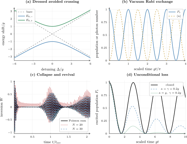
Generated benchmarks. (a) The $n=0$ dressed shifts avoid the crossing of the bare branches, with a resonant gap $2g$. (b) One excitation exchanges coherently between $|e,0\rangle$ and $|g,1\rangle$. (c) A coherent field with $\bar n=16$ shows unitary collapse and revival; the visibly displaced $N=20$ curve exposes an inadequate photon cutoff, while $N=30$ is closer but not converged to high precision. (d) Unconditional Lindblad loss damps the exchange and transfers weight to $|g,0\rangle$. Every curve is read from the downloadable CSV artifacts.

The figure is a summary, not a convergence certificate. In panel (c), the $N=40$ and $N=60$ curves would be visually indistinguishable from the Poisson sum at this scale, yet their numerical errors differ by nine orders of magnitude.

Verification Ladder

The calculation uses independent checks with different failure sensitivity.

Level 1: matrix identities

• $H=H^\dagger$;
• eigenvectors are orthonormal;
• analytic and numerical $2\times2$ eigenvalues agree; and
• resonance gaps follow $2g\sqrt{n+1}$.

These checks catch sign, square-root, and basis-order errors before time propagation.

Level 2: exact dynamics

• vacuum $P_e(t)=\cos^2(gt)$;
• vacuum $\langle n\rangle_t=\sin^2(gt)$;
• $P_e+\langle n\rangle=1$; and
• $\langle\mathcal N\rangle$ is constant.

Matching two complementary observables is stronger than matching one.

Level 3: representation convergence

• compute the omitted Poisson weight;
• repeat at increasing $N$;
• compare the target observable over the full time window; and
• compare with a structurally independent Poisson sum.

This level catches a perfectly unitary calculation in an inadequate basis.

Level 4: open-system physicality

• recover the closed limit;
• preserve trace;
• preserve Hermiticity;
• monitor the smallest density eigenvalue; and
• verify that loss reduces total excitation.

Trace preservation alone would not catch a nonpositive density matrix.

Error Ledger

Error source	Present in which calculation?	Diagnostic or control
two-level reduction	all	outside numerical convergence; compare with multilevel physics
rotating-wave approximation	all	outside cutoff convergence; compare with a Rabi-model extension
single-mode approximation	all	inspect cavity spectrum and coupling to other modes
photon cutoff	coherent-state runs	omitted tail plus observable convergence
top-edge blocking	coherent-state runs	compare with Poisson sum and raise $N$
floating-point diagonalization	closed runs	analytic spectra, norms, invariants
output-time sampling	revival peak report	refine sample grid or optimize locally
RK4 time step	loss extension	closed limit and step refinement
Markovian decay model	loss extension	model assumption, not a solver error
missing detector model	loss extension	do not call $\kappa\langle n\rangle$ a measured count record without efficiencies and filtering

Errors on different rows need different convergence campaigns. Increasing $N$ does not repair the rotating-wave approximation; decreasing the RK4 step does not add omitted cavity modes.

Program Architecture

The program separates physics construction from output and validation:

1. operator constructors build $a$, $a^\dagger a$, $H_I$, $H_{\mathrm{JC}}$, $\mathcal N$, and observables;
2. basis-state and coherent-state constructors define initial vectors;
3. a Hermitian spectral propagator evaluates all closed trajectories;
4. dedicated routines produce dressed, vacuum, revival, and cutoff rows;
5. a direct density-matrix RK4 routine produces the loss extension;
6. validators reject failed tolerances before metadata is written; and
7. CSV and JSON writers serialize deterministic outputs.

The code uses numpy.linalg.eigh for Hermitian matrices and numpy.linalg.eigvalsh for Hermitian density-matrix spectra. General eigensolvers would discard useful structure and can introduce avoidable complex roundoff into real eigenvalues.

Why diagonalization is appropriate here

For a time-independent Hermitian matrix, spectral propagation is:

• exact up to floating-point diagonalization and phase evaluation;
• unitary by construction to roundoff;
• efficient when many output times share one Hamiltonian; and
• easy to benchmark analytically.

It is not the default answer for:

• a strongly time-dependent drive;
• a very large sparse field basis;
• many emitters;
• a non-Hermitian generator; or
• a Liouvillian whose dense matrix scales as the square of Hilbert-space dimension.

The Time-Dependent Two-Level Systems Notebook develops explicit time stepping for driven Hamiltonians, while Solving Lindblad Equations maps broader open-system strategies.

Output schemas

The CSV artifacts preserve more than the plotted columns:

File	Selected columns
dressed spectrum	$\Delta/g$, both branch energies, centered shifts, atomic fractions, analytic shifts for $n=0,1$
vacuum Rabi	$gt$, $gt/\pi$, numerical and analytic $P_e$, numerical and analytic $\langle n\rangle$, total excitation
collapse–revival	$gt$, $t/t_{\mathrm{rev}}$, infinite-sum $W$, $P_e$, and all four finite-cutoff curves
truncation	$N$, highest $n$, omitted tail, errors versus $N=100$ and infinite sum, norm and excitation drift
loss	$gt$, $P_e$, $\langle n\rangle$, total excitation, $\kappa/g$, and $\gamma/g$ for every case

The metadata artifact records definitions and limitations that do not fit naturally into numeric columns. A figure can be regenerated without reverse-engineering its assumptions from line colors.

Reading the Results Responsibly

What is demonstrated

Within the declared model and tolerances, the outputs establish that:

• the tensor and manifold formulations agree;
• dressed doublets have the expected avoided crossings and square-root splittings;
• the vacuum exchanges one excitation coherently;
• a coherent photon-number distribution produces collapse and revival;
• the finite oscillator converges systematically for the selected observable and time window; and
• a small Lindblad extension recovers the closed limit and remains physical within its integration tolerance.

What is not demonstrated

The outputs do not establish:

• the validity of the two-level approximation for a particular emitter;
• the validity of the rotating-wave approximation at arbitrary $g/\omega_c$;
• strong coupling in a real device;
• a measured transmission or fluorescence spectrum;
• single-shot quantum jumps;
• nonclassicality from the inversion curve alone;
• convergence of a driven high-photon steady state; or
• agreement with an experiment that was not included in the model.

An avoided crossing is consistent with hybridization, but a measured avoided crossing needs a forward model including drive, damping, ports, and detector response before fitted parameters receive a cavity-QED interpretation.

Common Mistakes

Calling the cutoff the maximum photon number

In this notebook, $N$ is the field-space dimension. The largest retained number is $N-1$.

Checking only state norm

Renormalizing a truncated coherent state forces its norm to one. This says nothing about omitted probability.

Checking only the initial tail

Top-edge blocking can amplify observable error beyond the initial tail scale. Compare the observable itself.

Trusting a single cutoff

A single finite answer has no demonstrated representation convergence. Retain a sequence and a quantitative acceptance rule.

Swapping tensor order

kron(atom, field) and kron(field, atom) have the same dimensions but different index meanings. Projectors and initial states must use the same ordering as the Hamiltonian.

Missing the square root

The coupling in manifold $n$ is $g\sqrt{n+1}$, not $g(n+1)$ and not a constant $g$.

Confusing Rabi-frequency conventions

Here the resonance energy gap and population angular frequency in manifold $n$ are

$$\Omega_n=2g\sqrt{n+1}.$$

The vacuum excited population is $\cos^2(gt)$. A source that calls $g$ the Rabi frequency is using a different convention.

Calling unitary collapse decoherence

The collapse in the coherent-state curve results from reversible dephasing among number sectors. The revival is precisely the evidence that the phases were not irreversibly erased by the model.

Comparing incompatible detuning signs

This notebook uses $\Delta=\omega_a-\omega_c$. Translate formulas that use $\omega_c-\omega_a$ before comparing eigenvector composition or dispersive shifts.

Confusing energy and amplitude decay

With this page’s convention, $\kappa$ damps photon number as $e^{-\kappa t}$ and field amplitude as $e^{-\kappa t/2}$.

Using a no-jump Hamiltonian as an unconditional model

Non-Hermitian norm loss is a conditional survival probability. The unconditional master equation includes recycling terms.

Clipping density eigenvalues

Clipping can hide an unstable integrator. Report the minimum eigenvalue, refine the step, and use a suitable propagator if the violation is not negligible.

Extensions

Detuned exchange

Set $\Delta\ne0$ and compare the numerical one-excitation result with

$$P_e(t) = 1 - \frac{4g^2}{\Delta^2+4g^2} \sin^2 \left( \frac12 \sqrt{\Delta^2+4g^2}\,t \right).$$

This adds a simultaneous test of oscillation frequency and contrast.

Driven dissipative cavity

Adding a term such as

$$H_d = i\hbar \left( \eta a^\dagger-\eta^*a \right)$$

destroys excitation-number conservation and makes the photon cutoff dynamical. Convergence must then cover drive strength, transient duration, and steady-state photon distribution.

Input–output observables

A port-resolved model can connect the intracavity field to outgoing modes. Transmission, reflection, and detected count rates require coupling fractions, interference with incident fields, collection efficiency, bandwidth, and noise. Intracavity $\langle n\rangle$ alone is not a measured spectrum.

Beyond the rotating-wave approximation

Replace the interaction with the quantum Rabi form

$$H_{\mathrm{int}} = \hbar g \left( a+a^\dagger \right) \sigma_x.$$

Then $\mathcal N$ is not conserved, the ground state is dressed, and photon cutoff requirements change. Gauge consistency and diamagnetic terms can matter in ultrastrong-coupling regimes; this is a model change, not merely a larger matrix calculation.

Trajectory unraveling

The same Lindblad equation can be unraveled into stochastic quantum-jump records. Ensemble averages should recover the unconditional density matrix within sampling error. The Quantum-Jump Simulation page develops that numerical distinction.

Exercises

1. Prove excitation conservation

Show that

$$\mathcal N = a^\dagger a+\sigma_+\sigma_-$$

commutes with the Jaynes–Cummings Hamiltonian. Explain why this does not guarantee photon-cutoff convergence.

Solution

The free terms are functions of $a^\dagger a$ and $\sigma_z$, so they commute with $\mathcal N$. For the exchange terms, use

$$[a^\dagger a,a]=-a, \qquad [a^\dagger a,a^\dagger]=a^\dagger,$$

and

$$[\sigma_+\sigma_-,\sigma_+]=\sigma_+, \qquad [\sigma_+\sigma_-,\sigma_-]=-\sigma_-.$$

Then

$$\begin{aligned} [\mathcal N,a\sigma_+] &= -a\sigma_+ + a\sigma_+ =0,\\ [\mathcal N,a^\dagger\sigma_-] &= a^\dagger\sigma_- - a^\dagger\sigma_- =0. \end{aligned}$$

Hence $[H_{\mathrm{JC}},\mathcal N]=0$.

After truncation, the finite Hamiltonian can still commute with the finite version of $\mathcal N$. That identity tests internal consistency but not whether appreciable physical amplitude reaches the upper boundary. Cutoff convergence requires increasing $N$ and comparing the target observable.

2. Recover the dressed doublet

Diagonalize

$$B_n/\hbar = \frac12 \begin{pmatrix} \Delta&2g\sqrt{n+1}\\ 2g\sqrt{n+1}&-\Delta \end{pmatrix}$$

and find its resonant splitting.

Solution

The characteristic equation is

$$\det \left( \frac{B_n}{\hbar}-\varepsilon I \right) = \varepsilon^2 - \frac{\Delta^2}{4} - g^2(n+1) =0.$$

Thus

$$\varepsilon_{n,\pm} = \pm\frac12 \sqrt{\Delta^2+4g^2(n+1)}.$$

At $\Delta=0$,

$$\varepsilon_{n,\pm} = \pm g\sqrt{n+1},$$

so

$$E_{n,+}-E_{n,-} = 2\hbar g\sqrt{n+1}.$$

The common manifold center cancels from the splitting.

3. Verify vacuum Rabi exchange

Starting from $|e,0\rangle$ at resonance, derive the state and show that $P_e+\langle n\rangle=1$.

Solution

In the ordered basis $\{|e,0\rangle,|g,1\rangle\}$,

$$H_I/\hbar = \begin{pmatrix} 0&g\\ g&0 \end{pmatrix} = g\sigma_x.$$

Therefore

$$e^{-iH_It/\hbar} = \cos(gt)I-i\sin(gt)\sigma_x.$$

Acting on the first basis vector gives

$$|\psi(t)\rangle = \cos(gt)|e,0\rangle - i\sin(gt)|g,1\rangle.$$

Hence

$$P_e=\cos^2(gt), \qquad \langle n\rangle=\sin^2(gt),$$

and their sum is one. This equality expresses conservation of the single initial excitation.

4. Separate tail error from edge error

Let $q_N$ be the coherent-state probability above the cutoff. Show that the expectation of any observable $f_n\in[-1,1]$ under the renormalized conditional Poisson distribution differs from the full Poisson expectation by at most $2q_N$. Why can the finite Jaynes–Cummings matrix exceed this bound?

Solution

Write the full distribution as

$$P=(1-q_N)P_{\mathrm{in}}+q_NP_{\mathrm{out}},$$

where $P_{\mathrm{in}}$ is the normalized conditional distribution for $n<N$. Then

$$\langle f\rangle_P = (1-q_N)\langle f\rangle_{\mathrm{in}} + q_N\langle f\rangle_{\mathrm{out}}.$$

Therefore

$$\left| \langle f\rangle_{\mathrm{in}} - \langle f\rangle_P \right| = q_N \left| \langle f\rangle_{\mathrm{in}} - \langle f\rangle_{\mathrm{out}} \right| \le 2q_N.$$

This bound assumes that every retained component evolves with its correct function $f_n(t)$. The finite Jaynes–Cummings matrix violates that assumption for $|e,N-1\rangle$: its partner $|g,N\rangle$ is absent, so the upper-edge component has the wrong dynamics. The total finite-matrix error can therefore exceed $2q_N$, as the $N=30$ result does over part of the retained time window.

5. Estimate the revival time

Use the difference between neighboring Rabi frequencies near $\bar n$ to derive the leading revival time. Evaluate it for $\bar n=16$.

Solution

The resonant frequencies are

$$\Omega_n=2g\sqrt{n+1}.$$

Near a large $\bar n$,

$$\Omega_{n+1}-\Omega_n \approx \frac{d\Omega_n}{dn} \bigg|_{\bar n} \approx \frac{g}{\sqrt{\bar n}}.$$

Neighboring components rephase when

$$\left( \Omega_{n+1}-\Omega_n \right)t_{\mathrm{rev}} \approx 2\pi.$$

Thus

$$t_{\mathrm{rev}} \approx \frac{2\pi\sqrt{\bar n}}{g}.$$

For $\bar n=16$,

$$gt_{\mathrm{rev}} \approx 2\pi(4) = 8\pi \approx 25.1327.$$

The computed revival-envelope maximum occurs nearby, not exactly at this leading-order estimate.

6. Explain collapse without environmental decoherence

The atomic inversion nearly vanishes during the collapse region even though the full state is pure. Reconcile these statements.

Solution

The joint state has the schematic form

$$|\Psi(t)\rangle = \sum_n c_n \left[ \cos \left( g\sqrt{n+1}\,t \right)|e,n\rangle - i\sin \left( g\sqrt{n+1}\,t \right)|g,n+1\rangle \right].$$

Each number sector evolves coherently, and the joint state remains a unit vector produced by a unitary operator. The inversion is a weighted sum of oscillatory terms with different frequencies. Those terms dephase and cancel without losing their phases.

Tracing out the field can yield a mixed atomic density matrix because the atom is entangled with distinguishable field states. That is subsystem mixing, not impurity of the joint state. Later rephasing produces the revival, which would not occur under irreversible phase erasure in this closed model.

7. Derive the balanced-loss benchmark

For $\kappa=\gamma=\Gamma_d$ and no drive, show that

$$\langle\mathcal N(t)\rangle = e^{-\Gamma_dt} \langle\mathcal N(0)\rangle.$$

Solution

The Hamiltonian exchange conserves $\mathcal N$. A cavity jump $a$ removes one excitation whenever the excitation is photonic, and an emitter jump $\sigma_-$ removes one whenever it is atomic. The adjoint Lindblad equation therefore gives

$$\frac{d}{dt}\langle\mathcal N\rangle = -\kappa\langle a^\dagger a\rangle - \gamma \langle\sigma_+\sigma_-\rangle.$$

When $\kappa=\gamma=\Gamma_d$,

$$\frac{d}{dt}\langle\mathcal N\rangle = -\Gamma_d \left\langle a^\dagger a+\sigma_+\sigma_- \right\rangle = -\Gamma_d\langle\mathcal N\rangle.$$

Solving this scalar equation gives the stated exponential. With $\Gamma_d=0.2g$, $t=10/g$, and one initial excitation, the result is $e^{-2}=0.1353353$.

8. Design a positivity refinement test

The retained RK4 run has $\lambda_{\min}=-3.30\times10^{-12}$. Describe a test that distinguishes time-step error from a physical or implementation error.

Solution

Repeat the same calculation with maximum internal steps

$$h,\quad h/2,\quad h/4,$$

without clipping or renormalizing the density matrix. For each run retain:

• the minimum eigenvalue over time;
• the largest trace and Hermiticity errors;
• the maximum difference in $P_e(t)$ from the finest run; and
• the closed-limit analytic error.

In the asymptotic RK4 regime, observable differences should decrease by about $2^4=16$ when the step is halved. The small negative eigenvalue should move toward zero if it is a discretization artifact. Failure to converge, a violation that stays large, or a trace-preserving but increasingly negative state points to a generator, basis, or implementation error.

A completely positive exponential or splitting method provides a useful cross-formulation check, but agreement still needs time-step and representation tests.

9. Plan a driven-cavity cutoff campaign

Suppose a coherent cavity drive is added. Give an acceptance protocol for the photon cutoff that is stronger than requiring $\langle n\rangle\ll N$.

Solution

A defensible protocol should:

1. declare the drive, detuning, loss rates, initial state, time window, and target observables;
2. run an increasing sequence such as $N$, $N+\Delta N$, and $N+2\Delta N$;
3. compare the full time series or steady-state values of all reported observables;
4. inspect the upper-edge probability $\sum_{n=N-m}^{N-1}P_n$ for several edge states, not only the mean;
5. monitor trace, Hermiticity, positivity, and solver convergence independently;
6. require the changes to fall below a predeclared absolute or relative tolerance; and
7. retain the entire convergence record.

The condition $\langle n\rangle\ll N$ is insufficient because a broad or heavy-tailed distribution can have small mean relative to $N$ while still placing consequential weight at the boundary. Correlations and rare-event observables can converge more slowly than the mean photon number.

References

• E. T. Jaynes and F. W. Cummings, “Comparison of quantum and semiclassical radiation theories with application to the beam maser,” Proceedings of the IEEE 51, 89–109 (1963). Original model and quantum–semiclassical comparison.
• J. H. Eberly, N. B. Narozhny, and J. J. Sanchez-Mondragon, “Periodic spontaneous collapse and revival in a simple quantum model,” Physical Review Letters 44, 1323–1326 (1980). Original collapse–revival result.
• G. Rempe, H. Walther, and N. Klein, “Observation of quantum collapse and revival in a one-atom maser,” Physical Review Letters 58, 353–356 (1987). First experimental observation of the predicted revival.
• B. W. Shore and P. L. Knight, “The Jaynes–Cummings model,” Journal of Modern Optics 40, 1195–1238 (1993). Detailed review of analytic dynamics and extensions.
• H. Walther, B. T. H. Varcoe, B.-G. Englert, and T. Becker, “Cavity quantum electrodynamics,” Reports on Progress in Physics 69, 1325–1382 (2006). Review of one-atom maser theory and experiments.
• S. Haroche and J.-M. Raimond, Exploring the Quantum: Atoms, Cavities, and Photons, Oxford University Press (2006). Graduate treatment of cavity QED and atom–field dynamics.
• H. J. Carmichael, Statistical Methods in Quantum Optics 1: Master Equations and Fokker–Planck Equations, Springer (1999). Open-system and quantum-optical master-equation methods.
• H.-P. Breuer and F. Petruccione, The Theory of Open Quantum Systems, Oxford University Press (2002). General Lindblad dynamics and approximations.
• A. Blais, A. L. Grimsmo, S. M. Girvin, and A. Wallraff, “Circuit quantum electrodynamics,” Reviews of Modern Physics 93, 025005 (2021). Modern review of Jaynes–Cummings, dispersive, driven, and dissipative physics in circuit QED.
• NumPy developers, numpy.linalg.eigh documentation. Hermitian eigensolver used by the executable artifact.

Further Study

• Continue to Laser Cooling before building the next AMO computation, where internal dynamics are coupled to motion through a velocity-dependent scattering force.
• Reproducibility Benchmarks cross-checks the resonant doublets, vacuum exchange, producer validations, runtime record, and artifact identity.
• Use the Computational AMO and Quantum Chemistry overview to compare the Jaynes–Cummings splitting with the chapter’s atomic, molecular, and driven-system benchmark ladder.
• Return to Cavity QED before attaching these dimensionless calculations to a measured cavity linewidth, cooperativity, or output spectrum.