Laser Cooling Simulation Notebook

A velocity-dependent force is not yet a cooling prediction. Cooling requires a restoring force in velocity space, a momentum-diffusion model, a declared convention for that diffusion coefficient, and evidence that the numerical operations reproduce the analytic limits they are supposed to represent.

This notebook constructs that evidence for a deliberately small model. It computes:

1. the two directional radiation-pressure forces and their net force;
2. weak-field force curves for red and blue detuning;
3. the low-velocity friction coefficient by both analysis and finite differences;
4. a fourth-order convergence test for the numerical derivative;
5. the friction–diffusion equilibrium temperature and its optimum detuning;
6. a declared shared-saturation extension that exposes intensity tradeoffs;
7. a friction–diffusion relaxation benchmark with an exact solution; and
8. a representative rubidium-87 D2 conversion from dimensionless to SI scales.

The retained headline results are:

Diagnostic	Computed value	What it tests
largest force-oddness error	$5.55\times10^{-17}$	balanced-beam symmetry
largest directional-sum error	$6.94\times10^{-18}$	component bookkeeping
largest analytic–numeric friction error	$1.07\times10^{-11}$	five-point derivative
detuning for maximum weak friction	$0.288675131\,\Gamma$	numerical optimization
detuning for minimum weak temperature	$0.499999996\,\Gamma$	friction–diffusion balance
minimum weak temperature	$1.000000000\,T_D$	Doppler-limit identity
smallest five-point derivative error	$6.25\times10^{-11}$	refinement study
largest relaxation error	$1.37\times10^{-10}$	RK4 against exact moments
rubidium-87 D2 Doppler scale	$145.537\,\mu\mathrm K$	SI conversion

The two optimum detunings differ. Maximum local damping occurs at $\Delta/\Gamma=1/(2\sqrt3)$, whereas minimum equilibrium temperature occurs at $\Delta/\Gamma=1/2$. Optimizing the force slope alone does not optimize a cooling process because recoil diffusion changes with detuning too.

Run the investigation. The program and retained results below support the stated experiment. Follow Running an Experiment for environment and output-directory guidance. The recorded evidence applies to its stated parameters and environment.

Purpose and Canonical Scope

This page is the canonical home for an executable, deterministic benchmark of simple Doppler cooling. Its responsibilities are to:

• make detuning, linewidth, saturation, force, velocity, and diffusion conventions machine-readable;
• expose the two signed beam forces before summing them;
• compare a numerical derivative with the analytic friction coefficient;
• demonstrate the expected fourth-order finite-difference regime;
• verify the relation $k_{\mathrm B}T=D_p/\alpha$ in one declared geometry;
• separate the weak-field result from a finite-intensity toy extension;
• distinguish damping time, equilibrium temperature, and force range;
• convert one dimensionless benchmark to representative atomic scales; and
• export every curve and validation result as CSV or JSON.

Neighboring pages retain distinct canonical responsibilities:

• Laser Cooling owns the broad taxonomy of Doppler, polarization-gradient, narrow-line, Raman, sideband, and related cooling mechanisms.
• Doppler Cooling owns the complete textbook derivation of the scattering force, friction, recoil-diffusion ledger, Doppler temperature, capture range, and experimental limitations.
• Radiation Pressure owns the general momentum-transfer and scattering-force derivation.
• Optical Bloch Equations owns the internal-state dynamics from which steady-state two-level scattering rates follow.
• Optical Bloch Equation Notebook verifies those internal-state transients, steady states, and emitted-power proxies without center-of-mass motion.
• Sub-Doppler Cooling owns multilevel mechanisms that can invalidate the two-level Doppler temperature as an experimental floor.

The present page does not repeat those derivations. It turns one controlled subset into an auditable numerical object.

Reproducibility Contract

The executable artifact is a NumPy-only Python program:

• Download the program
• Force-curve data
• Friction data
• Temperature data
• Intensity-scan data
• Derivative-convergence data
• Relaxation data
• Rubidium-scale data
• Machine-readable metadata and validation

Run the downloaded program from the folder where you saved it:

python laser-cooling-simulation.py --output-dir results

The default run declares:

Item	Choice
language	Python 3
numerical dependency	NumPy
random numbers	none
force samples	$1201$
friction samples	$801$
temperature samples	$1001$
intensity samples	$241$
relaxation samples	$501$
derivative stencil	five-point centered
relaxation integrator	classical explicit RK4
largest internal RK4 step	$0.005$ normalized time unit
canonical detuning	$\Delta=\omega_0-\omega_L$
red detuning	$\Delta>0$
linewidth	angular decay rate $\Gamma$
saturation	on-resonance value for one beam
force normalization	$\hbar k\Gamma$
velocity coordinate	$u=kv/\Gamma$
diffusion convention	$d\,\operatorname{Var}(p_x)/dt=2D_p$

Odd sample counts retain both endpoints and the central sample. The program uses no random seed, fit, adaptive optimizer, plotting package, or external AMO library. A deterministic golden-section search locates smooth scalar optima. The JSON artifact records runtime versions, equations, limits, source identifiers, all validation booleans, and all output names.

Claim boundary

The main calculation assumes:

• a closed two-level transition;
• two balanced, counterpropagating plane waves;
• equal frequency, intensity, and polarization response for the two beams;
• weak saturation when independent scattering rates are added;
• a local internal steady state at each velocity;
• classical, nonrelativistic center-of-mass motion;
• dilute, noninteracting particles; and
• three orthogonal beam pairs with isotropic spontaneous emission for the retained three-dimensional diffusion ledger.

The finite-intensity curves replace the weak denominator by one explicit shared-saturation denominator. They are labeled a representative two-level extension, not an exact multi-beam optical Bloch solution.

The model excludes hyperfine and Zeeman sublevels, optical pumping, polarization gradients, coherent standing-wave effects, dark states, magnetic trapping, gravity, spatial beam profiles, branching loss, collisions, reabsorption, density-dependent radiation pressure, laser noise, stochastic trajectories, and sub-Doppler mechanisms. Consequently, the rubidium calculation is a scale conversion for an idealized closed transition, not a quantitative molasses or magneto-optical-trap prediction.

Dimensionless Interface and Sign Convention

Define

$$u=\frac{kv}{\Gamma}, \qquad d=\frac{\Delta}{\Gamma}, \qquad \Delta=\omega_0-\omega_L.$$

Here $k>0$ is the beam wave number, $v$ is the atomic velocity along $+x$, and $\Gamma$ is an angular-frequency linewidth. In this convention:

$$\text{red detuning}\quad\Longleftrightarrow\quad d>0.$$

Many papers and software packages instead define

$$\delta=\omega_L-\omega_0=-\Delta.$$

For that convention red detuning means $\delta<0$. The friction CSV exports both Delta_over_Gamma and delta_laser_minus_atom_over_Gamma; changing notation should negate a column, not silently change the physics.

The force is reported as

$$f(u;d,s) = \frac{F(v)}{\hbar k\Gamma},$$

where $s$ is the on-resonance saturation parameter of one beam. A dimensionless force curve is species-independent only after all of these definitions are fixed.

Why angular frequency matters

The Doppler shift $kv$, detuning $\Delta$, and linewidth $\Gamma$ in the formulas are angular frequencies. If a tabulation gives the natural linewidth as $\Gamma/(2\pi)$ in hertz, the conversion is

$$\Gamma = 2\pi \left(\frac{\Gamma}{2\pi}\right)_{\mathrm{Hz}}.$$

Using a linewidth in hertz beside $kv$ in radians per second creates a factor-of-$2\pi$ error in velocity, force, damping time, and temperature.

Weak Counterpropagating Force

The program evaluates the two signed force components

$$\begin{aligned} f_+(u) &= \frac{s}{2} \frac{1}{1+4(d+u)^2}, \\ f_-(u) &= -\frac{s}{2} \frac{1}{1+4(d-u)^2}, \end{aligned}$$

and then adds them:

$$f(u) = \frac{s}{2} \left[ \frac{1}{1+4(d+u)^2} - \frac{1}{1+4(d-u)^2} \right].$$

The sign attached to $f_-$ is mechanical: absorption from the $-x$ beam transfers momentum $-\hbar k$. The two Lorentzians by themselves are nonnegative scattering rates; their signed momenta produce the net force.

Symmetry checks

Balanced beams imply

$$f(-u)=-f(u)$$

and therefore

$$f(0)=0.$$

The generated grid gives

$$\max_u|f(u)+f(-u)| = 5.55\times10^{-17},$$

and exactly zero net force at the retained central sample. It also verifies the component identity

$$f_+(u)+f_-(u)=f(u)$$

to $6.94\times10^{-18}$.

These are strong implementation checks because they test indexing, signs, and normalization. They are not evidence that the physical assumptions are appropriate for a particular atom.

Red and blue detuning

For small positive velocity and red detuning,

$$d>0,\quad u>0 \quad\Longrightarrow\quad f(u)<0.$$

The force opposes the motion. At $d=-1/2$, the same scan gives $f(u)>0$ near the origin: blue detuning antidamps the motion in this two-level model.

The force file retains curves at

$$d\in\left\{-\frac12,\frac14,\frac12,1,2\right\}$$

over $-3\le u\le3$, plus the two directional components at $d=1/2$. Keeping a blue-detuned curve is useful: a sign error can otherwise produce a plausible-looking red-only plot.

Force range is not a capture theorem

The counterpropagating force has substantial structure near velocity classes for which one beam approaches resonance. A useful scale is

$$|u|\sim d, \qquad |v|\sim\frac{\Delta}{k}.$$

This is a resonant-velocity or force-range proxy. It is not, by itself, a capture velocity. Capture depends on interaction length, initial position, acceleration over the full trajectory, beam profile, level structure, branching, and any external force. The notebook intentionally does not turn one force-curve maximum into an apparatus claim.

Low-Velocity Friction

Near the origin, write

$$F(v) = -\alpha v + O(v^3).$$

Because the balanced force is odd, no quadratic term appears. In normalized variables,

$$\frac{\alpha}{\hbar k^2} = - \left. \frac{\partial f}{\partial u} \right|_{u=0}.$$

Differentiating the weak force gives

$$\frac{\alpha_{\mathrm w}}{\hbar k^2} = \frac{8sd}{(1+4d^2)^2}.$$

Thus $\alpha_{\mathrm w}>0$ for red detuning and $\alpha_{\mathrm w}<0$ for blue detuning. The program checks those signs at every nonzero sample in $-2\le d\le2$.

Numerical derivative

The independent numerical estimate uses the five-point centered stencil

$$f'(0) \approx \frac{ f(-2h)-8f(-h)+8f(h)-f(2h) }{ 12h }.$$

The friction estimate is $-\hbar k^2 f'(0)$. For a smooth force, the truncation error is $O(h^4)$ until floating-point cancellation becomes important.

At the production step $h=10^{-3}$, the largest disagreement across the friction scan is

$$\max_d \left| \frac{\alpha_{\mathrm{num}}-\alpha_{\mathrm{exact}}} {\hbar k^2} \right| = 1.07\times10^{-11}.$$

The analytic and numerical columns remain separate in the CSV. A validation test should not overwrite the quantity it is meant to check.

Refinement study

The convergence artifact evaluates the derivative at $d=1/2$, $s=0.1$, where

$$\frac{\alpha}{\hbar k^2}=0.1.$$

It uses

$$h\in \{0.08,0.04,0.02,0.01,0.005,0.0025\}.$$

For fourth-order convergence, halving $h$ should reduce the leading error by approximately

$$2^4=16.$$

The observed refinement ratios range from $15.9485$ to $16.0006$. The finest retained error is $6.25\times10^{-11}$. This verifies the expected asymptotic regime; it does not imply that indefinitely smaller steps are better. Eventually roundoff in nearly equal force values dominates.

Maximum damping

At fixed weak saturation, maximizing

$$a(d)=\frac{8sd}{(1+4d^2)^2}$$

over $d>0$ gives

$$d_{\alpha,\mathrm{opt}} = \frac{1}{2\sqrt3} \approx 0.288675135.$$

The numerical optimizer returns

$$d_{\alpha,\mathrm{num}} = 0.288675131,$$

an absolute location error of $3.35\times10^{-9}$. This is the detuning for the steepest local force slope, not the detuning for the lowest friction–diffusion equilibrium.

Momentum Diffusion and Temperature

The canonical Doppler Cooling page derives the recoil ledger. The notebook consumes one explicit result rather than silently choosing a factor of two.

It defines $D_p$ by

$$\frac{d}{dt} \operatorname{Var}(p_x) = 2D_p$$

and adopts three orthogonal weak beam pairs with isotropic spontaneous emission. For one Cartesian axis, the retained weak-field model is

$$\frac{D_p}{\hbar^2k^2\Gamma} = \frac{s}{1+4d^2}.$$

This coefficient includes the absorption-number fluctuations and the projected spontaneous-emission recoil appropriate to the declared three-dimensional ledger. A one-dimensional emission model or a convention with $d\,\operatorname{Var}(p_x)/dt=D_p$ would produce a different numerical coefficient.

Friction–diffusion balance

For the Ornstein–Uhlenbeck momentum model,

$$dp = -\frac{\alpha}{m}p\,dt + \sqrt{2D_p}\,dW_t,$$

the stationary variance is

$$\operatorname{Var}(p) = \frac{mD_p}{\alpha}.$$

Using equipartition along one axis,

$$\operatorname{Var}(p)=mk_{\mathrm B}T,$$

gives

$$k_{\mathrm B}T = \frac{D_p}{\alpha}.$$

With

$$k_{\mathrm B}T_D = \frac{\hbar\Gamma}{2},$$

the dimensionless weak-field temperature becomes

$$\frac{T}{T_D} = \frac{1+4d^2}{4d}.$$

The program independently evaluates $\alpha$, $D_p$, and $T/T_D$ and checks

$$\frac{T}{T_D} = 2 \frac{ D_p/(\hbar^2k^2\Gamma) }{ \alpha/(\hbar k^2) }$$

over all $1001$ temperature samples. The largest identity error is $1.78\times10^{-15}$.

Minimum temperature

Minimizing the weak expression gives

$$d_{T,\mathrm{opt}} = \frac12, \qquad T_{\min}=T_D.$$

The numerical search returns

$$d_{T,\mathrm{num}} = 0.499999996, \qquad \frac{T_{\min,\mathrm{num}}}{T_D} = 1.$$

This equality is a property of the declared two-level, weak-field, semiclassical model. It is not a universal lower bound on laser cooling. Multilevel polarization-gradient mechanisms famously produce temperatures below this value, while technical noise and nonideal geometry can produce temperatures above it.

Why weak-field intensity cancels

In the weak model,

$$\alpha\propto s, \qquad D_p\propto s.$$

Therefore their ratio, and hence the equilibrium temperature, is independent of $s$. Lower intensity does not make the weak-model temperature colder. It reduces both damping and diffusion, lengthening the approach to equilibrium.

That cancellation holds only while the same linear-in-$s$ approximation is valid for both quantities. It should not be extrapolated into strong saturation or multilevel optical pumping.

A Controlled Saturation Extension

To expose power broadening without claiming a complete multi-beam solution, the notebook also defines

$$b=1+2s,$$

where $s$ remains the saturation parameter per beam, and uses

$$f_{\mathrm{sh}}(u) = \frac{s}{2} \left[ \frac{1}{b+4(d+u)^2} - \frac{1}{b+4(d-u)^2} \right].$$

The subscript “sh” denotes the declared shared-saturation denominator. It does not denote a unique or exact theory of saturated optical molasses.

Within this extension,

$$\frac{\alpha_{\mathrm{sh}}}{\hbar k^2} = \frac{8sd}{(b+4d^2)^2},$$

and

$$\frac{D_{p,\mathrm{sh}}}{\hbar^2k^2\Gamma} = \frac{s}{b+4d^2}.$$

The corresponding temperature model is

$$\frac{T_{\mathrm{sh}}}{T_D} = \frac{b+4d^2}{4d}.$$

Analytic optima

For fixed $s$, minimizing the shared temperature gives

$$d_{\mathrm{sh,opt}} = \frac{\sqrt{1+2s}}{2},$$

and

$$\frac{T_{\mathrm{sh,min}}}{T_D} = \sqrt{1+2s}.$$

The numerical optimizer verifies both identities at

$$s\in\{0.01,0.1,0.5,2\}.$$

The largest retained location error is $2.13\times10^{-8}$, and the largest temperature-value error is $4.44\times10^{-16}$.

Detuning and intensity tradeoffs

The intensity artifact scans

$$10^{-3}\le s\le10$$

at $241$ logarithmically spaced points. For each point it reports:

• friction at fixed $d=1/2$;
• temperature at fixed $d=1/2$;
• the temperature-optimal detuning;
• the minimum temperature in the shared model;
• friction at that temperature optimum;
• the positive-velocity location of the force extremum; and
• the magnitude of that extremum as a force-range proxy.

Across the scan, the peak normalized force grows from $4.02\times10^{-4}$ to $6.52\times10^{-2}$, while the optimized shared-model temperature grows from $1.0010\,T_D$ to $4.5826\,T_D$.

This illustrates a genuine design tension even though the quantitative extension is only representative:

• greater intensity can increase available force and broaden the velocity response;
• power broadening shifts the favorable detuning;
• stronger scattering increases momentum diffusion; and
• the coldest setting need not provide the fastest preparation or largest force range.

A real multilevel calculation must replace the shared denominator with a specified master equation, polarization geometry, magnetic field, and branching structure.

Relaxation Benchmark

The static temperature formula checks an equilibrium ratio. It does not verify time evolution. The notebook therefore integrates the moment equations of the same linear friction–diffusion model.

Define the velocity damping time

$$\tau_v=\frac{m}{\alpha}$$

and normalized time

$$\tau=\frac{t}{\tau_v}.$$

The normalized mean velocity $\mu$ and temperature ratio $\theta=T/T_{\mathrm{eq}}$ obey

$$\frac{d\mu}{d\tau} = -\mu,$$

and

$$\frac{d\theta}{d\tau} = -2(\theta-1).$$

The exact solutions are

$$\mu(\tau) = \mu_0e^{-\tau},$$

and

$$\theta(\tau) = 1+(\theta_0-1)e^{-2\tau}.$$

The variance relaxes twice as fast as the mean because it is quadratic in the fluctuating velocity.

Numerical cases

Classical RK4 is tested on:

1. $\mu_0=1$ for mean-velocity damping;
2. $\theta_0=10$ for cooling from above equilibrium; and
3. $\theta_0=0$ for recoil heating from an artificially cold initial state.

Over $0\le\tau\le5$, the largest errors are:

Quantity	Largest absolute error
normalized mean	$7.35\times10^{-13}$
hot temperature	$1.37\times10^{-10}$
cold temperature	$1.52\times10^{-11}$

The program also checks that the hot case decreases monotonically and the cold case increases monotonically.

The cold curve matters conceptually. Diffusion is not a correction that can be omitted once an atom is slow. In this model, a distribution narrower than equilibrium heats toward the same stationary variance.

What this time evolution omits

The relaxation equations use the force linearized at $v=0$ and a constant diffusion coefficient. They cannot describe initial velocities near or beyond the nonlinear force range, spatial escape, changing internal states, or velocity-dependent diffusion. A full trajectory calculation would integrate the nonlinear force and specify a stochastic recoil process.

Rubidium-87 Scale Conversion

The dimensionless benchmark is converted using a representative rubidium-87 D2 transition:

Input	Retained value
wavelength $\lambda$	$780.241209686\,\mathrm{nm}$
linewidth $\Gamma/(2\pi)$	$6.065\,\mathrm{MHz}$
mass $m$	$1.44316060\times10^{-25}\,\mathrm{kg}$
saturation per beam $s$	$0.1$
red detuning $\Delta/\Gamma$	$0.5$

The wavelength and linewidth are representative values from Daniel Steck’s Rubidium 87 D Line Data. Fundamental constants use exact SI values where applicable, as collected by NIST. The mass value is retained explicitly in the program rather than fetched at runtime.

The conversion uses

$$k=\frac{2\pi}{\lambda}, \qquad \Gamma = 2\pi(6.065\,\mathrm{MHz}).$$

At $d=1/2$,

$$T_D = \frac{\hbar\Gamma}{2k_{\mathrm B}} = 145.537\,\mu\mathrm K.$$

The recoil scale is

$$T_r = \frac{\hbar^2k^2}{2mk_{\mathrm B}} = 0.180978\,\mu\mathrm K.$$

Thus

$$\frac{T_D}{T_r} \approx 804.17.$$

The semiclassical Doppler scale lies far above one recoil temperature for this broad transition.

Velocity and time scales

The one-recoil velocity is

$$v_r = \frac{\hbar k}{m} = 5.8845\times10^{-3}\,\mathrm{m\,s^{-1}}.$$

The one-dimensional rms speed at $T_D$ is

$$v_{\mathrm{rms},D} = \sqrt{\frac{k_{\mathrm B}T_D}{m}} = 0.1180\,\mathrm{m\,s^{-1}}.$$

The resonant-velocity scale at $d=1/2$ is

$$v_{\mathrm{res}} = \frac{\Delta}{k} = 2.3661\,\mathrm{m\,s^{-1}}.$$

For $s=0.1$, the weak friction coefficient is

$$\alpha = 6.839\times10^{-22}\,\mathrm{kg\,s^{-1}},$$

so

$$\tau_v = \frac{m}{\alpha} = 0.2110\,\mathrm{ms}.$$

The normalized pair-force curve reaches a magnitude corresponding to $1.304\times10^{-21}\,\mathrm N$ in the retained scan. The single-beam two-level ceiling $\hbar k\Gamma/2$ is $1.618\times10^{-20}\,\mathrm N$.

These scales are internally consistent. They are not expected to reproduce the temperature, loading rate, damping time, or capture velocity of a real rubidium apparatus without its hyperfine repumping, polarization, magnetic-field, beam-profile, and technical-noise model.

Benchmark Figure

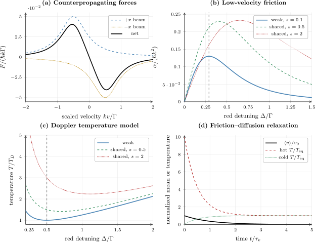
Deterministic outputs of the retained model. (a) The two signed beam forces cancel at zero velocity and produce an odd damping force for $\Delta/\Gamma=1/2$ and $s=0.1$. (b) The weak-field friction maximum occurs at $\Delta/\Gamma=1/(2\sqrt3)$; shared-saturation curves are controlled extensions, not multilevel molasses predictions. (c) The weak friction–diffusion temperature is minimized at $\Delta/\Gamma=1/2$, while shared saturation raises and shifts the model minimum. (d) Mean velocity relaxes on $\tau_v=m/\alpha$ and temperature on $\tau_v/2$; both hot and artificially cold initial variances approach the same equilibrium.

Verification Ladder

The program uses checks at several logically distinct levels.

Level 1: algebraic identities

It verifies:

$$f(-u)=-f(u), \qquad f(0)=0, \qquad f_++f_-=f.$$

These checks detect sign, indexing, and component-sum mistakes.

Level 2: physical sign tests

For small positive $u$, it requires:

$$d>0\Longrightarrow f(u)<0,$$

and

$$d<0\Longrightarrow f(u)>0.$$

The corresponding friction coefficient must be positive for red detuning and negative for blue detuning.

Level 3: analytic comparisons

The numerical derivative is compared with the closed friction formula. The optimizer is compared with analytic friction and temperature optima. The independently assembled friction–diffusion ratio is compared with the closed temperature expression.

Level 4: convergence

A six-step refinement campaign verifies decreasing derivative error and an approximately $16$-fold reduction under step halving. A single small discrepancy would not establish the stencil’s order.

Level 5: dynamical benchmarks

RK4 trajectories are compared pointwise with exact mean and variance relaxation. Monotonicity checks distinguish cooling from recoil heating.

Level 6: dimensional plausibility

The rubidium conversion checks broad expected ranges for Doppler temperature, recoil temperature, damping time, and resonant velocity. These tests catch unit errors, especially missing factors of $2\pi$, but they do not validate an apparatus.

Error Ledger

Error source	Controlled here by	Residual limitation
detuning-sign error	dual sign columns and red/blue tests	external sources may use another convention
beam-momentum sign error	exported directional forces	assumes perfect counterpropagation
derivative truncation	analytic comparison and step refinement	roundoff eventually limits smaller $h$
interpolation error	direct formulas on retained grids	plotted lines interpolate between samples
scalar optimization error	analytic optimum comparisons	only smooth one-dimensional objectives
time-integration error	exact relaxation solutions	only linear moment equations are tested
diffusion factor error	explicit variance convention and geometry	other geometries have other coefficients
saturation-model error	separate label and formula	not an exact multi-beam Bloch calculation
atomic-data error	retained source and literal constants	not a critical evaluation of every datum
model discrepancy	explicit exclusions	dominant for real multilevel experiments

The smallest floating-point residual is not necessarily the most important error. For a real cooling experiment, omitted level structure and optical pumping can dominate numerical errors by many orders of magnitude.

Program Architecture

The program keeps the physics layers small and independently testable:

1. weak_force evaluates the balanced weak-field force.
2. weak_directional_forces exposes the signed beam contributions.
3. shared_saturation_force evaluates the declared power-broadened extension.
4. analytic_friction evaluates the exact origin slope.
5. numerical_friction applies the five-point stencil.
6. normalized_diffusion supplies the declared three-dimensional ledger.
7. doppler_temperature_ratio forms the equilibrium ratio.
8. golden_section_minimum performs deterministic scalar optimization.
9. rk4_relaxation propagates normalized mean and temperature moments.
10. dataset builders assemble CSV rows and their validation records.
11. the main routine rejects invalid sample counts, writes artifacts, and refuses to emit successful metadata if any check fails.

Every CSV floating-point field is written with $16$ significant digits. JSON serialization converts NumPy scalar types explicitly. No validation field is inferred later from a plotted image.

Output schemas

laser-cooling-force-curves.csv contains:

• $u=kv/\Gamma$;
• the $+x$ and $-x$ beam forces at $d=1/2$, $s=0.1$;
• their net force;
• weak net-force curves for five detunings; and
• shared-saturation force curves for four intensities.

laser-cooling-friction.csv contains:

• both detuning sign conventions;
• analytic and five-point weak friction; and
• shared-saturation friction for four intensities.

laser-cooling-temperature.csv contains:

• red detuning and $2\Delta/\Gamma$;
• weak temperature, friction, and diffusion;
• the independently reconstructed $2D_p/\alpha$ ratio; and
• shared-saturation temperatures.

laser-cooling-intensity.csv contains:

• per-beam and total saturation;
• fixed-detuning friction and temperature;
• temperature-optimal detuning and temperature;
• friction at the temperature optimum; and
• force-extremum location and magnitude.

laser-cooling-convergence.csv contains:

• derivative step;
• numerical and analytic friction;
• absolute error; and
• the refinement ratio to the next step.

laser-cooling-relaxation.csv contains numerical and exact values for:

• normalized mean velocity;
• cooling from $10T_{\mathrm{eq}}$; and
• heating from zero initial variance.

laser-cooling-rubidium.csv is one transparent SI-scale record. The JSON file contains all conventions, validation thresholds and outcomes, scope limits, source identifiers, runtime versions, and output names.

Reading the Results Responsibly

What is demonstrated

Within the declared model, the artifacts demonstrate that:

• balanced weak-beam forces have the required odd symmetry;
• red detuning damps and blue detuning antidamps near zero velocity;
• the numerical force derivative reproduces analytic friction;
• the five-point stencil reaches its fourth-order convergence regime;
• maximum friction and minimum temperature occur at different detunings;
• the weak-field Doppler minimum follows from friction–diffusion balance;
• shared saturation produces force–temperature tradeoffs in the declared extension;
• both hot and cold momentum variances relax toward one equilibrium; and
• the dimensionless benchmark converts consistently to rubidium scales.

What is not demonstrated

The artifacts do not demonstrate:

• an experimentally universal temperature floor;
• sub-Doppler cooling;
• a capture velocity for a finite apparatus;
• magneto-optical trapping or positional confinement;
• a valid saturated multi-beam master equation;
• an exact stochastic momentum distribution;
• quantitative rubidium hyperfine dynamics;
• molecular optical cycling;
• robustness to intensity, frequency, polarization, or magnetic-field noise; or
• agreement with a measured cooling curve.

The distinction between a validated implementation and a validated physical model is essential. This notebook establishes the former for a narrow theory benchmark.

Common Mistakes

Reversing the detuning sign

With $\Delta=\omega_0-\omega_L$, red detuning is positive. A formula copied from a source using $\delta=\omega_L-\omega_0$ must be translated before interpreting a force sign.

Forgetting the momentum sign of one beam

Both scattering rates are positive. The force from the $-x$ beam is negative because the absorbed photon momentum is $-\hbar k$.

Mixing hertz and radians per second

The tabulated $\Gamma/(2\pi)$ in hertz must be multiplied by $2\pi$ before using it with $kv$ or $\hbar\Gamma/(2k_{\mathrm B})$.

Calling zero net force a trap

Balanced molasses has $F(0)=0$ and damps velocity, but the homogeneous model has no positional restoring force. A magneto-optical trap adds spatially varying Zeeman shifts and polarization selection.

Computing temperature from friction alone

Positive $\alpha$ establishes damping of the mean. The equilibrium temperature requires a momentum-diffusion ledger with an explicit convention.

Dropping spontaneous recoil because its mean is zero

The mean projected recoil can vanish while its variance grows. Diffusion is set by the second moment.

Hiding the factor of two in diffusion

The statement $d\,\operatorname{Var}(p)/dt=2D_p$ is not interchangeable with $d\,\operatorname{Var}(p)/dt=D_p$. The temperature formula must match the chosen definition.

Optimizing only the force slope

The fastest weak local damping occurs at $d=1/(2\sqrt3)$. The coldest weak equilibrium occurs at $d=1/2$ because diffusion changes with detuning.

Treating a force maximum as capture velocity

A force curve lacks the interaction distance and trajectory information needed to decide whether an atom actually stops before leaving the beams.

Adding saturated rates independently

At finite intensity, beams share the same atomic population and coherence. Independent saturated Lorentzians can double-count excitation. The notebook’s shared denominator is explicit precisely so it cannot be mistaken for a unique exact theory.

Calling the Doppler scale universal

Alkali atoms are multilevel systems. Polarization-gradient cooling can produce temperatures below the two-level Doppler value; technical effects can produce higher temperatures.

Shrinking the derivative step without a convergence plot

Truncation error decreases with $h$, but cancellation and floating-point roundoff eventually increase. A refinement campaign is more informative than one impressively small step.

Extensions

Nonlinear stochastic trajectories

Replace the linear moment model with

$$m\,dv = F(v)\,dt + \sqrt{2D_p(v)}\,dW_t.$$

A credible extension should compare an ensemble Fokker–Planck or stochastic simulation with the linear analytic limit, report time-step and ensemble convergence separately, and avoid interpreting a single noisy trajectory as a temperature.

Full multi-beam optical Bloch model

Promote the local scattering formula to a master equation with both driving fields. Declare polarization, relative optical phase, rotating-wave convention, branching structure, and whether spatial standing-wave coherences are retained. Recover the weak independent-beam force before using the model at high saturation.

Hyperfine and Zeeman structure

Add magnetic sublevels, Clebsch–Gordan coefficients, optical pumping, repumping light, magnetic fields, and polarization gradients. The resulting force can depend on position and internal history as well as velocity.

Magneto-optical trapping

Include spatial Zeeman shifts and beam helicities so the drift has both velocity and position dependence:

$$F(x,v) \approx -\kappa x-\alpha v.$$

Benchmark the damping and trap frequencies separately, then test gravity, beam imbalance, finite beam size, and loss.

Narrow-line and recoil-resolved regimes

When $\hbar\Gamma$ approaches the recoil energy, continuous momentum diffusion and semiclassical motion become questionable. A momentum-state master equation or quantum-jump treatment can retain discrete recoil.

Parameter inference

To compare with data, add an observation model and independently measured calibrations. Fit force or cooling curves only after specifying likelihood, uncertainties, nuisance parameters, and identifiability. A deterministic forward curve alone is not an error bar.

Exercises

1. Translate the detuning convention

A library defines $\delta=\omega_L-\omega_0$ and reports red detuning $\delta/\Gamma=-0.7$. Convert this to the convention of the notebook. For an atom with small positive velocity, state the expected sign of the force and friction.

Solution

The notebook uses

$$\Delta=\omega_0-\omega_L=-\delta.$$

Therefore

$$\frac{\Delta}{\Gamma} = -\frac{\delta}{\Gamma} = 0.7.$$

This is red detuning in the notebook convention. Near $v=0$,

$$F(v)\approx-\alpha v.$$

For $\Delta>0$, the weak formula gives $\alpha>0$. Hence a small positive velocity produces $F<0$: the force opposes the motion.

2. Prove the force symmetry

Starting from the weak normalized force, show that $f(-u)=-f(u)$ and $f(0)=0$. Explain one experimental condition whose violation would remove this odd symmetry.

Solution

Write

$$f(u) = \frac{s}{2} \left[ \frac{1}{1+4(d+u)^2} - \frac{1}{1+4(d-u)^2} \right].$$

Replacing $u$ by $-u$ interchanges the two denominators:

$$\begin{aligned} f(-u) &= \frac{s}{2} \left[ \frac{1}{1+4(d-u)^2} - \frac{1}{1+4(d+u)^2} \right] \\ &=-f(u). \end{aligned}$$

Setting $u=0$ then gives $f(0)=-f(0)$, so $f(0)=0$. Unequal beam intensities, unequal detunings, imperfect counterpropagation, or different polarization coupling can break the symmetry and produce a nonzero force at zero velocity.

3. Recover the five-point convergence ratio

The centered five-point derivative has leading error $Ch^4$. What error ratio should be observed when $h$ is halved? Why should this ratio eventually fail as $h$ becomes extremely small?

Solution

At step $h$, the leading truncation error is

$$\epsilon(h)\approx Ch^4.$$

At half the step,

$$\epsilon(h/2) \approx C\left(\frac h2\right)^4 = \frac{\epsilon(h)}{16}.$$

Therefore

$$\frac{\epsilon(h)}{\epsilon(h/2)} \approx16.$$

The stencil subtracts nearly equal force values and divides by $h$. As $h$ becomes very small, floating-point representation and cancellation errors are amplified. The total error then ceases to follow $Ch^4$ and can grow under further refinement.

4. Find the maximum-friction detuning

For fixed $s>0$, maximize

$$a(d)=\frac{8sd}{(1+4d^2)^2}$$

over $d>0$.

Solution

The constant factor $8s$ does not affect the optimum. Differentiate:

$$\begin{aligned} \frac{d}{dd} \left[ d(1+4d^2)^{-2} \right] &= (1+4d^2)^{-2} - 16d^2(1+4d^2)^{-3} \\ &= \frac{1-12d^2}{(1+4d^2)^3}. \end{aligned}$$

The positive stationary point satisfies

$$1-12d^2=0,$$

so

$$d_{\alpha,\mathrm{opt}} = \frac{1}{2\sqrt3}.$$

The derivative changes from positive to negative there, and $a(d)$ tends to zero at both $d\to0^+$ and $d\to\infty$, so this stationary point is the global maximum.

5. Find the Doppler-temperature minimum

Minimize

$$\frac{T}{T_D} = \frac{1+4d^2}{4d}$$

for $d>0$. Compare the result with Exercise 4.

Solution

Rewrite the ratio as

$$\frac{T}{T_D} = \frac{1}{4d}+d.$$

Then

$$\frac{d}{dd} \left( \frac{1}{4d}+d \right) = -\frac{1}{4d^2}+1.$$

The positive stationary point is

$$d=\frac12.$$

The second derivative $1/(2d^3)$ is positive, so this is a minimum. Its value is

$$\left.\frac{T}{T_D}\right|_{d=1/2} = \frac12+\frac12 = 1.$$

This differs from the maximum-friction point $1/(2\sqrt3)\approx0.2887$. Friction and diffusion have different detuning dependence.

6. Audit the diffusion convention

Suppose another source defines $\widetilde D_p$ by

$$\frac{d}{dt}\operatorname{Var}(p)=\widetilde D_p$$

instead of the notebook convention $d\,\operatorname{Var}(p)/dt=2D_p$. Express $\widetilde D_p$ in terms of $D_p$ and write the temperature formula using $\widetilde D_p$.

Solution

Equating the two variance-growth rates gives

$$\widetilde D_p=2D_p.$$

The notebook equilibrium formula is

$$k_{\mathrm B}T=\frac{D_p}{\alpha}.$$

Substituting $D_p=\widetilde D_p/2$ gives

$$k_{\mathrm B}T = \frac{\widetilde D_p}{2\alpha}.$$

Using $k_{\mathrm B}T=\widetilde D_p/\alpha$ without translating the definition would overestimate the temperature by a factor of two.

7. Optimize the shared-saturation model

For $b=1+2s$, minimize

$$g(d)=\frac{b+4d^2}{4d}$$

over $d>0$. Evaluate the optimum detuning and minimum temperature at $s=1/2$.

Solution

Rewrite

$$g(d) = \frac{b}{4d}+d.$$

Then

$$g'(d) = -\frac{b}{4d^2}+1.$$

The positive optimum is

$$d_{\mathrm{opt}} = \frac{\sqrt b}{2} = \frac{\sqrt{1+2s}}{2}.$$

At this point,

$$g_{\min} = \sqrt b = \sqrt{1+2s}.$$

For $s=1/2$, $b=2$, so

$$d_{\mathrm{opt}} = \frac{1}{\sqrt2} \approx0.7071,$$

and

$$\frac{T_{\min}}{T_D} = \sqrt2 \approx1.4142.$$

These are properties of the declared shared-denominator extension, not universal saturated-molasses values.

8. Compare mean and temperature relaxation

How long, in units of $\tau_v$, does it take the mean velocity to fall to $1\%$ of its initial value? How long does a temperature excess $T-T_{\mathrm{eq}}$ take to fall to $1\%$ of its initial excess?

Solution

The mean obeys

$$\frac{\mu(\tau)}{\mu_0}=e^{-\tau}.$$

Setting this ratio to $0.01$ gives

$$\tau_\mu = \ln 100 \approx4.6052.$$

The temperature excess obeys

$$\frac{ T(\tau)-T_{\mathrm{eq}} }{ T(0)-T_{\mathrm{eq}} } = e^{-2\tau}.$$

Setting this ratio to $0.01$ gives

$$\tau_T = \frac12\ln100 \approx2.3026.$$

Thus the variance or temperature excess relaxes twice as rapidly as the mean in normalized time.

9. Diagnose a linewidth-unit error

An implementation inserts $6.065\times10^6\,\mathrm{s^{-1}}$ directly for $\Gamma$ in the rubidium Doppler formula, although $6.065\,\mathrm{MHz}$ was the tabulated value of $\Gamma/(2\pi)$. What Doppler temperature does it obtain, and by what factor is it wrong?

Solution

The incorrect calculation uses

$$T_D^{\mathrm{wrong}} = \frac{ \hbar(6.065\times10^6\,\mathrm{s^{-1}}) }{ 2k_{\mathrm B} }.$$

The correct angular linewidth is

$$\Gamma = 2\pi(6.065\times10^6\,\mathrm{s^{-1}}).$$

Therefore

$$T_D^{\mathrm{wrong}} = \frac{T_D^{\mathrm{correct}}}{2\pi}.$$

Using the retained correct value,

$$T_D^{\mathrm{wrong}} = \frac{145.537\,\mu\mathrm K}{2\pi} \approx 23.16\,\mu\mathrm K.$$

The result is too small by a factor of $2\pi$. The same mistake would shrink the converted resonant velocity and force scale and alter the damping-time conversion.

References

1. T. W. Hänsch and A. L. Schawlow, “Cooling of Gases by Laser Radiation,” Optics Communications 13, 68–69 (1975), doi:10.1016/0030-4018(75)90159-5.
2. S. Chu, L. Hollberg, J. E. Bjorkholm, A. Cable, and A. Ashkin, “Three-Dimensional Viscous Confinement and Cooling of Atoms by Resonance Radiation Pressure,” Physical Review Letters 55, 48–51 (1985), doi:10.1103/PhysRevLett.55.48.
3. S. Stenholm, “The Semiclassical Theory of Laser Cooling,” Reviews of Modern Physics 58, 699–739 (1986), doi:10.1103/RevModPhys.58.699.
4. P. D. Lett, R. N. Watts, C. I. Westbrook, W. D. Phillips, P. L. Gould, and H. J. Metcalf, “Observation of Atoms Laser Cooled below the Doppler Limit,” Physical Review Letters 61, 169–172 (1988), doi:10.1103/PhysRevLett.61.169.
5. J. Dalibard and C. Cohen-Tannoudji, “Laser Cooling below the Doppler Limit by Polarization Gradients: Simple Theoretical Models,” Journal of the Optical Society of America B 6, 2023–2045 (1989), doi:10.1364/JOSAB.6.002023.
6. W. D. Phillips, “Laser Cooling and Trapping of Neutral Atoms,” Reviews of Modern Physics 70, 721–741 (1998), doi:10.1103/RevModPhys.70.721.
7. H. J. Metcalf and P. van der Straten, Laser Cooling and Trapping (Springer, 1999), doi:10.1007/978-1-4612-1470-0.
8. C. J. Foot, Atomic Physics (Oxford University Press, 2005), publisher record.
9. D. A. Steck, “Rubidium 87 D Line Data,” version 2.3.4, revised 8 August 2025, Alkali D Line Data.
10. National Institute of Standards and Technology, “CODATA Values of the Fundamental Constants,” Constants, Units, and Uncertainty.

Further Study

• Doppler Cooling derives the physical model and its diffusion ledger in full.
• Laser Cooling places Doppler cooling among the major cooling mechanisms.
• Sub-Doppler Cooling explains why real multilevel atoms can cool below the two-level Doppler scale.
• Radiation Pressure develops scattering forces and recoil from first principles.
• Optical Bloch Equation Notebook verifies the internal steady-state response used by force models.
• Convergence Tests develops refinement ratios, observed order, and error-floor diagnostics.
• Reproducibility Benchmarks independently checks force signs, oddness, friction and temperature optima, producer validations, runtime record, and artifact identity.
• Notebook Index catalogs executable artifacts and their reproducibility contracts.