Scattering Theory

Scattering theory connects quantum dynamics to collision experiments. An incoming state is prepared far from an interaction region, the interaction redistributes amplitude among possible outgoing channels, and detectors measure rates as functions of angle, energy, momentum transfer, spin, or internal state.

The central objects form a hierarchy:

$$\begin{gathered} \text{Hamiltonian} \longrightarrow \text{scattering state} \\ \longrightarrow \text{amplitude} \longrightarrow \text{cross section}. \end{gathered}$$

The same process can be organized by an $S$-matrix between asymptotic states, a $T$-matrix of transition amplitudes, a Lippmann–Schwinger integral equation, or phase shifts in angular-momentum channels. These are not competing definitions. They are representations adapted to different questions.

This volume uses nonrelativistic three-dimensional potential scattering as its main language. The canonical amplitude convention is in Scattering Amplitude, observable counting is in Differential and Total Cross Sections, and the operator construction begins at Lippmann–Schwinger Equation.

Enter this volume

1. Scattering States and Observables connects preparations, amplitudes, and measured cross sections.
2. Scattering Operators and Unitarity develops exact operators and scattering-specific Born expansions.
3. Partial Waves and Threshold Scattering uses symmetry and low-energy parameters.
4. Poles, Resonances, and Scattering Channels interprets states and channel structure.

Use the worked problems and computational studies alongside those chapters. General approximation principles belong to Approximation and Semiclassical Methods; operator-theoretic existence and completeness questions belong to Mathematical Quantum Mechanics.

What Scattering Theory Computes

A scattering problem begins with an incoming channel $\alpha$. A channel specifies the asymptotic particle content and every conserved or measured label needed to define free motion: momentum, internal state, spin, threshold, and sometimes target state.

The interaction can produce an outgoing channel $\beta$. The differential cross section is the outgoing rate divided by incident flux:

$$d\sigma_{\beta\leftarrow\alpha} = \frac{ dR_{\beta\leftarrow\alpha} }{ j_\alpha }.$$

This ratio has units of area. It removes the arbitrary intensity of the incident beam and characterizes how effectively the target redirects flux into a specified final region.

Common distinctions are:

• elastic scattering: the asymptotic internal channel is unchanged and kinetic energy is conserved;
• inelastic scattering: internal excitation, reaction, or another open channel changes the outgoing kinetic energy;
• fixed-target potential scattering: one particle moves in a prescribed potential;
• two-body scattering: center-of-mass motion separates and the relative coordinate uses the reduced mass;
• single-channel scattering: only one asymptotic channel is open;
• multichannel scattering: elastic, inelastic, open, and closed channels are coupled.

The cross section is not the probability of an isolated normalized state. Plane waves describe steady incident flux, and cross sections compare outgoing rate with that flux. Wave packets provide the more physical preparation, while stationary states supply the energy-resolved formulas.

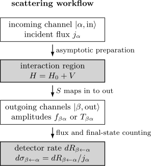
The Hamiltonian determines the map from an asymptotic incoming channel $\alpha$ to outgoing channels $\beta$. The complex amplitude carries phase information; combining it with incident flux and final-state counting produces the observable differential cross section.

Incoming and Outgoing Asymptotic States

Let

$$H=H_0+V,$$

where $H_0$ describes free relative motion and $V$ is a short-range interaction. For one elastic channel with incident momentum $\mathbf k$, the outgoing stationary state has the large-distance form

$$\begin{aligned} \psi_{\mathbf k}^{(+)}(\mathbf r) \sim{}& e^{i\mathbf k\cdot\mathbf r} \\ &+ f(\mathbf k'\leftarrow\mathbf k) \frac{e^{ikr}}{r}, \\ &\quad \mathbf k'=k\hat{\mathbf r}. \end{aligned}$$

The first term is the incident plane wave. The second is an outgoing spherical wave. Its coefficient

$$f(\mathbf k'\leftarrow\mathbf k)$$

is the scattering amplitude. For a central potential and an incident beam chosen along $z$, rotational symmetry reduces it to $f(\theta)$.

The superscript $(+)$ denotes the outgoing boundary condition on the scattered wave. It does not mean positive energy. The incoming solution $\psi^{(-)}$ uses the opposite boundary condition and is needed in formal matrix elements.

At the operator level, the Møller wave operators are formally

$$\Omega^{(\pm)} = \lim_{t\to\mp\infty} e^{iHt/\hbar} e^{-iH_0t/\hbar}.$$

They turn free asymptotic states into interacting scattering states:

$$\lvert\psi_\alpha^{(\pm)}\rangle = \Omega^{(\pm)} \lvert\phi_\alpha\rangle.$$

Their existence and completeness require assumptions. Bound states are not scattering states, long-range interactions can require modified asymptotic dynamics, and rigorous asymptotic completeness is a theorem only for suitable Hamiltonians.

Unscreened Coulomb scattering is the standard warning. Its long-range phase does not fit the simple plane-wave-plus-spherical-wave asymptotic form without modification. Coulomb Scattering owns that case.

Flux, Amplitude, and Cross Section

For a scalar Schrödinger wavefunction with mass $m$, the probability current is

$$\mathbf j = \frac{\hbar}{2mi} \left( \psi^*\nabla\psi - \psi\nabla\psi^* \right).$$

A unit-amplitude incident plane wave carries flux

$$j_{\mathrm{inc}} = \frac{\hbar k}{m}.$$

The outgoing spherical wave carries radial flux proportional to

$$\frac{\lvert f(\theta,\phi)\rvert^2}{r^2}.$$

Multiplication by the detector area element $r^2d\Omega$ cancels geometric spreading. For single-channel elastic scattering in the convention above,

$$\frac{d\sigma}{d\Omega} = \lvert f(\theta,\phi)\rvert^2.$$

Thus $f$ has dimensions of length and $d\sigma/d\Omega$ has dimensions of area. The total elastic cross section is

$$\sigma_{\mathrm{el}} = \int d\Omega\, \lvert f(\theta,\phi)\rvert^2.$$

For a transition from channel $\alpha$ to $\beta$, outgoing and incoming speeds can differ:

$$\frac{d\sigma_{\beta\leftarrow\alpha}}{d\Omega} = \frac{v_\beta}{v_\alpha} \lvert f_{\beta\alpha}\rvert^2.$$

Identical particles require amplitudes for indistinguishable alternatives to be added before taking the modulus squared. Identical-Particle Scattering develops exchange interference, spin dependence, and one-count-per-pair phase-space bookkeeping. Detector acceptance, target recoil, and channel thresholds also belong in the observable definition.

When the outgoing internal state differs from the incoming one, Inelastic Scattering Preview specializes the velocity factor, Q-value bookkeeping, channel sums, and golden-rule connection.

S-Matrix and T-Matrix

The scattering operator maps the remote past to the remote future:

$$S = \Omega^{(-)\dagger} \Omega^{(+)}.$$

Its matrix elements compare asymptotic channels:

$$S_{\beta\alpha} = \langle\phi_\beta\lvert S \rvert\phi_\alpha\rangle.$$

The identity part describes no scattering. The remainder is conventionally expressed through a transition operator $T$. One common energy-normalized convention is schematic:

$$S_{\beta\alpha} = \delta_{\beta\alpha} - 2\pi i\, \delta(E_\beta-E_\alpha) T_{\beta\alpha}.$$

Factors of $2\pi$, $\hbar$, volume, velocity, and delta functions depend on state normalization. A formula for $T$ is meaningful only together with its normalization convention.

S-Matrix owns the wave-operator construction and energy-shell structure. Unitarity owns the resulting channel constraints, partial-wave disk, and cross-section bounds. T-Matrix owns the transition operator, normalization ledger, and on-shell versus off-shell distinction. Born Series owns its order-by-order expansion and convergence.

For outgoing boundary conditions, the transition operator satisfies

$$T(E) = V + V G_0^{(+)}(E)T(E),$$

where

$$G_0^{(+)}(E) = \frac{1}{E-H_0+i0}.$$

Green Function for Scattering shows how this boundary value becomes an outgoing coordinate kernel, how its far-field phase projects onto the energy shell, and how a localized source becomes the scattering amplitude.

The scattering amplitude is proportional to the on-shell matrix element

$$\langle\mathbf k'\lvert T(E) \rvert\mathbf k\rangle,$$

with the proportionality factor fixed by normalization. “On shell” means

$$E = \frac{\hbar^2k^2}{2m} = \frac{\hbar^2k'^2}{2m}$$

for elastic scattering.

Unitarity,

$$S^\dagger S=I,$$

expresses conservation of total probability across all open channels. In the standard amplitude convention it implies the optical theorem

$$\sigma_{\mathrm{tot}} = \frac{4\pi}{k} \operatorname{Im}f(0).$$

The forward elastic amplitude therefore knows about the total rate removed from the incident beam, including inelastic channels when they are present. Unitarity develops the operator and channel constraints; Optical Theorem owns this forward-amplitude identity and its convention checks.

Lippmann–Schwinger and the Born Route

The outgoing scattering state satisfies

$$\lvert\psi^{(+)}\rangle = \lvert\phi\rangle + G_0^{(+)}V \lvert\psi^{(+)}\rangle.$$

This is exact. Iterating it gives the Born series:

$$\begin{aligned} \lvert\psi^{(+)}\rangle ={}& \lvert\phi\rangle + G_0^{(+)}V\lvert\phi\rangle \\ &+ G_0^{(+)}V G_0^{(+)}V\lvert\phi\rangle + \cdots . \end{aligned}$$

Equivalently,

$$\begin{aligned} T ={}& V+VG_0^{(+)}V \\ &+ VG_0^{(+)}VG_0^{(+)}V +\cdots . \end{aligned}$$

The displayed iteration is formal until a convergence criterion or finite-order error argument is supplied. Born Series develops the second term, perturbative unitarity, remainder bounds, and pole-driven failure.

The first Born approximation replaces the exact scattering state inside the interaction region by the incident plane wave. With this chapter’s convention,

$$f_{\mathrm B}(\mathbf q) = - \frac{m}{2\pi\hbar^2} \int d^3r\, e^{-i\mathbf q\cdot\mathbf r} V(\mathbf r),$$

where

$$\mathbf q=\mathbf k'-\mathbf k.$$

It turns scattering into a Fourier probe of a weak potential. First Born Approximation owns the derivation and worked transforms. Validity of the Born Approximation owns weak-coupling and high-energy criteria, threshold and long-range warnings, and numerical tests.

Partial Waves and Phase Shifts

For a central potential, angular momentum is conserved and the problem separates into independent $\ell$ channels. The amplitude is

$$\begin{aligned} f(\theta) = \frac{1}{k} \sum_{\ell=0}^{\infty} (2\ell+1) e^{i\delta_\ell} \sin\delta_\ell\, P_\ell(\cos\theta). \end{aligned}$$

The phase shift $\delta_\ell$ measures the change in asymptotic radial phase relative to free motion. The partial-wave $S$-matrix is

$$S_\ell=e^{2i\delta_\ell}$$

for elastic scattering. Its unit modulus is channel-by-channel unitarity. Unitarity develops the corresponding Argand disk, inelasticity parameter, and partial-wave bounds.

The total elastic cross section is

$$\sigma_{\mathrm{el}} = \frac{4\pi}{k^2} \sum_{\ell=0}^{\infty} (2\ell+1) \sin^2\delta_\ell.$$

At low energy, the centrifugal barrier suppresses large $\ell$. For a finite-range potential of range $R$, the rough number of important partial waves is

$$\ell_{\max}\sim kR.$$

When $kR\ll1$, the $s$-wave often dominates. Partial-Wave Expansion owns the angular decomposition, Phase Shifts owns their interpretation and extraction, and Partial-Wave Cross Sections owns the channel sums, threshold hierarchy, and worked examples.

Threshold Physics

For short-range interactions at low energy, detailed potential structure becomes difficult to resolve. The leading $s$-wave amplitude is organized by the scattering length $a$:

$$f_0(k) \simeq \frac{1}{ -a^{-1}-ik }.$$

The next correction is encoded by the effective range $r_e$:

$$k\cot\delta_0(k) = - \frac{1}{a} + \frac{1}{2}r_e k^2 + O(k^4).$$

This is an expansion in momentum and analyticity, not a weak-potential expansion. A potential can be strong while its low-energy scattering remains describable by a few threshold parameters.

Low-Energy Scattering owns the universal regime, Scattering Length owns definitions and sign conventions, and Effective-Range Expansion owns the systematic threshold series.

Bound States, Resonances, and Poles

The same Hamiltonian controls bound and scattering states. Their unity becomes especially clear after analytically continuing amplitudes or the $S$-matrix away from real positive energy.

• A bound state appears as a pole at negative real energy on the physical sheet.
• A virtual state is a nearby non-normalizable pole on a different sheet or momentum-axis location.
• A resonance is associated with a pole at complex energy and produces a finite lifetime.

For an isolated resonance, the pole energy is commonly written

$$E_{\mathrm{pole}} = E_R-\frac{i}{2}\Gamma,$$

with lifetime scale

$$\tau\sim\frac{\hbar}{\Gamma}.$$

A peak in a cross section can signal a resonance, but background interference, thresholds, overlapping poles, and channel coupling can distort or hide the peak. A Breit–Wigner fit is a model with a domain of validity, not the definition of a resonance.

Bound States and Scattering Poles owns the analytic continuation, while Resonances owns phase-shift, width, lifetime, and lineshape diagnostics.

Choosing a Scattering Method

Regime or question	Natural first route	Primary output	Main warning
weak short-range potential	First Born Approximation	Fourier-space amplitude	repeated scattering and resonances
central potential at general strength	Partial-Wave Expansion	phase shifts $\delta_\ell$	enough partial waves must be retained
short-range threshold scattering	Low-Energy Scattering	$a$, $r_e$, shallow poles	expansion fails above the range scale
unscreened $1/r$ interaction	Coulomb Scattering	Coulomb amplitude and phases	ordinary short-range asymptotics fail
identical outgoing particles	Identical-Particle Scattering	direct–exchange amplitude and spatial parity	final pairs must be counted once
narrow structure in energy	Resonances	pole, phase motion, width	background and thresholds matter
isolated narrow-resonance line shape	Breit–Wigner Form	unitary pole factor and partial widths	nearby singularities deform the profile
several internal thresholds	Multichannel Scattering Preview	channel $S$-matrix	closed channels still shift open ones
resolved internal-energy transfer	Inelastic Scattering Preview	channel-resolved differential cross section	Q-values and velocity ratios must be explicit
one-dimensional leads and barriers	One-Dimensional Scattering Revisited	reflection, transmission, and two-channel $S$	transfer conventions and evanescent conditioning matter
infer an interaction from data	Inverse Scattering Preview	constrained potential or phase data	uniqueness requires assumptions
translate to relativistic reactions	Bridge to QFT Scattering	invariant amplitude and phase space	normalization and kinematics change

Born and partial-wave methods are not mutually exclusive. Born theory can estimate phase shifts, and a partial-wave calculation can benchmark a perturbative amplitude. The best method is the one whose control parameter, symmetry reduction, and observable are explicit.

Convention Ledger

Before comparing scattering formulas, record:

Choice	Why it matters
time dependence $e^{-iEt/\hbar}$	fixes outgoing and incoming Green-function signs
plane-wave normalization	moves factors among $f$, $T$, delta functions, and cross sections
fixed target or center-of-mass frame	determines whether $m$ is a particle mass or reduced mass
short-range or long-range interaction	determines the correct asymptotic states
distinguishable or identical particles	determines amplitude symmetrization
elastic or multichannel problem	determines velocity factors and unitarity sums
lab or center-of-mass angle	changes kinematic conversion of measured distributions
spin resolved, summed, or averaged	changes the reported observable

Most apparent contradictions between scattering formulas are convention mismatches. The cure is to compare the asymptotic wave, state normalization, and cross-section definition before comparing coefficients.

Reading Route

For a first pass:

1. Begin with What Is a Scattering Experiment?, then define the continuum states at Scattering States and Boundary Conditions.
2. Follow the conserved flow at Probability Current and Flux, then connect it to Scattering Amplitude and Differential and Total Cross Sections.
3. Organize the asymptotic channels with S-Matrix, isolate the transition amplitudes at T-Matrix, learn the exact state equation at Lippmann–Schwinger Equation, and follow its source to the detector at Green Function for Scattering.
4. Study repeated interactions and convergence at Born Series, derive the leading formula at First Born Approximation, and test its domain at Validity of the Born Approximation. Use Partial-Wave Expansion, Phase Shifts, and Partial-Wave Cross Sections when central-potential channels require nonperturbative control.
5. Organize probability-conservation constraints at Unitarity, then use Optical Theorem for the forward-amplitude check.
6. Continue to Low-Energy Scattering, Scattering Length, and Effective-Range Expansion for threshold physics.
7. Add Bound States and Scattering Poles and Resonances for analytic structure, then use Breit–Wigner Form for an isolated narrow-resonance parameterization.
8. Add Coulomb Scattering for long-range dynamics and Identical-Particle Scattering for exchange-sensitive observables.
9. Use One-Dimensional Scattering Revisited to translate the canonical barrier models into full scattering language. Finish with Multichannel Scattering Preview and Inelastic Scattering Preview for channel-changing collisions, then continue to Inverse Scattering Preview and Bridge to QFT Scattering.

Page Map

Page	Canonical role
What Is a Scattering Experiment?	beam, target, detector, luminosity, and data reduction
Scattering States and Boundary Conditions	incident data, radiation conditions, and continuum normalization
Probability Current and Flux	incident, scattered, interference, and channel-flux bookkeeping
Scattering Amplitude	asymptotic wave and amplitude convention
Differential and Total Cross Sections	flux-to-observable conversion
S-Matrix	asymptotic operator map, energy-shell channels, and unitarity
T-Matrix	transition operator, normalization, and shell structure
Lippmann–Schwinger Equation	exact resolvent integral equation for scattering states
Green Function for Scattering	outgoing free kernel, far-field factorization, and amplitude extraction
Born Series	repeated interactions, convergence, and perturbative unitarity
First Born Approximation	weak-potential Fourier-transform approximation
Validity of the Born Approximation	range, strength, energy, pole, and numerical validity tests
Partial-Wave Expansion	angular-momentum channel decomposition
Phase Shifts	physical and numerical phase-shift interpretation
Partial-Wave Cross Sections	elastic, reaction, and total channel sums, bounds, thresholds, and examples
Optical Theorem	forward-amplitude consequence of unitarity
Unitarity	channel sum rules, partial-wave disk, and cross-section bounds
Low-Energy Scattering	short-range threshold universality
Scattering Length	leading $s$-wave threshold parameter
Effective-Range Expansion	systematic low-momentum expansion
Bound States and Scattering Poles	analytic continuation and pole classification
Resonances	quasibound states, widths, signatures, and physical classification
Breit–Wigner Form	pole factor, phase motion, line shape, partial widths, and validity limits
Coulomb Scattering	long-range asymptotics and Rutherford result
Identical-Particle Scattering	exchange interference, spin symmetry, event counting, and partial-wave selection
Multichannel Scattering Preview	thresholds, channel matrices, and Feshbach resonances
Inelastic Scattering Preview	internal-state energy transfer, flux factors, and transition-rate bridge
One-Dimensional Scattering Revisited	left/right channels, transfer matrices, poles, resonant tunneling, and WKB comparison
Inverse Scattering Preview	reconstruction and uniqueness caveats
Bridge to QFT Scattering	relativistic amplitudes, phase space, and LSZ preview

QFT Bridge

The durable concepts are asymptotic in and out states, complex amplitudes, flux-normalized observables, unitarity, thresholds, poles, and resonances. Relativistic quantum field theory changes the realization:

• interactions are generated by fields and a Lagrangian or Hamiltonian density rather than a prescribed potential;
• Lorentz-invariant phase space replaces fixed-energy solid-angle counting;
• particle number can change;
• spin, crossing, internal quantum numbers, and identical-particle statistics become integral to the amplitude;
• LSZ reduction connects time-ordered correlation functions to scattering amplitudes.

The nonrelativistic formula

$$\frac{d\sigma}{d\Omega} = \lvert f\rvert^2$$

should not be inserted into a relativistic calculation. Its conceptual architecture survives, but normalization and kinematics must be rebuilt. The canonical translation is Bridge to QFT Scattering.

Common Mistakes

• Treating the scattering amplitude as a probability rather than a complex amplitude.
• Forgetting that cross sections are rates divided by incident flux.
• Calling the $(+)$ state positive energy rather than outgoing.
• Comparing $T$-matrix formulas without matching state normalization.
• Using short-range asymptotic formulas for an unscreened Coulomb potential.
• Applying the Born approximation near a resonance because the potential looks simple.
• Keeping too few partial waves when $kR$ is large.
• Treating a cross-section peak as the definition of a resonance.
• Ignoring velocity ratios, channel sums, or identical-particle interference.
• Confusing a fixed-target laboratory angle with a center-of-mass angle.
• Assuming that every formal scattering state is square normalizable.

Cross-Links

• Free Particle
• Probability Current
• Continuity Equation
• Normalization Conventions
• Energy Green Function
• Green Function for Scattering
• Born Series
• Spherical Harmonics
• Fermi’s Golden Rule
• QFT Bridge: S-Matrix
• QFT Bridge: Optical Theorem and Unitarity

References

1. B. A. Lippmann and J. Schwinger, “Variational principles for scattering processes. I,” Physical Review 79, 469–480 (1950).
2. J. R. Taylor, Scattering Theory: The Quantum Theory of Nonrelativistic Collisions, Dover (2006).
3. R. G. Newton, Scattering Theory of Waves and Particles, 2nd ed., Dover (2002).
4. M. L. Goldberger and K. M. Watson, Collision Theory, Dover (2004).
5. C. J. Joachain, Quantum Collision Theory, 3rd ed., North-Holland (1983).
6. M. Reed and B. Simon, Methods of Modern Mathematical Physics, Vol. III: Scattering Theory, Academic Press (1979).
7. J. J. Sakurai and J. Napolitano, Modern Quantum Mechanics, 3rd ed., Cambridge University Press (2020).
8. S. Weinberg, The Quantum Theory of Fields, Vol. I: Foundations, Cambridge University Press (1995).

Exercises

Dimensions from flux

In three dimensions, an outgoing spherical wave is

$$\psi_{\mathrm{sc}} = f(\theta,\phi) \frac{e^{ikr}}{r}.$$

Use the ratio of outgoing rate through $r^2d\Omega$ to incident flux to explain why $f$ has dimensions of length.

Solution

The radial scattered current scales as

$$j_r^{\mathrm{sc}} \sim v \frac{\lvert f\rvert^2}{r^2},$$

where $v=\hbar k/m$. The outgoing rate through an area element is

$$dR \sim j_r^{\mathrm{sc}}r^2d\Omega = v\lvert f\rvert^2d\Omega.$$

Dividing by incident flux $j_{\mathrm{inc}}=v$ gives

$$\frac{d\sigma}{d\Omega} = \lvert f\rvert^2.$$

A cross section has units of area, so $f$ must have units of length.

Choose the first method

Choose a natural first method for each problem: a weak Gaussian potential at high energy, a hard sphere at arbitrary strength, a short-range potential at $kR\ll1$, and an unscreened Coulomb potential.

Solution

• The weak high-energy Gaussian suggests the first Born approximation.
• The central hard sphere suggests partial waves and exact boundary matching.
• The short-range threshold problem suggests $s$-wave scattering length and effective-range methods.
• The unscreened Coulomb problem requires Coulomb asymptotics rather than the ordinary short-range framework.

Each choice follows from a different organizing feature: weak coupling, rotational symmetry, low momentum, or long range.

Elastic s-wave unitarity

For one elastic $s$-wave,

$$f_0 = \frac{1}{k} e^{i\delta_0} \sin\delta_0.$$

Show that

$$\operatorname{Im}f_0 = k\lvert f_0\rvert^2$$

and verify the optical theorem.

Solution

The modulus is

$$\lvert f_0\rvert^2 = \frac{\sin^2\delta_0}{k^2}.$$

The imaginary part is

$$\operatorname{Im}f_0 = \frac{\sin^2\delta_0}{k}.$$

Therefore

$$\operatorname{Im}f_0 = k\lvert f_0\rvert^2.$$

The total $s$-wave cross section is

$$\sigma_0 = 4\pi\lvert f_0\rvert^2 = \frac{4\pi}{k} \operatorname{Im}f_0,$$

which is the optical theorem for an isotropic elastic amplitude.

Partial-wave unitarity bound

Use

$$\sigma_\ell = \frac{4\pi}{k^2} (2\ell+1) \sin^2\delta_\ell$$

to find the largest possible elastic contribution from one partial wave.

Solution

Since

$$0\le\sin^2\delta_\ell\le1,$$

the maximum occurs at

$$\delta_\ell = \frac{\pi}{2} \pmod{\pi}.$$

Thus

$$\sigma_\ell \le \frac{4\pi}{k^2} (2\ell+1).$$

This is the elastic partial-wave unitarity bound in the stated convention.

Pole of the zero-range amplitude

Consider

$$f_0(k) = \frac{1}{-a^{-1}-ik}.$$

For $a\gt0$, locate the pole in the complex $k$-plane and find its energy using reduced mass $\mu$.

Solution

The denominator vanishes when

$$- \frac{1}{a} - ik = 0,$$

so

$$k=\frac{i}{a}.$$

This pole lies on the positive imaginary $k$-axis and corresponds to a shallow bound state. Its energy is

$$E = \frac{\hbar^2k^2}{2\mu} = - \frac{\hbar^2}{2\mu a^2}.$$

Finite-range corrections change this relation when $a$ is not much larger than the interaction range.