One-Dimensional Scattering Revisited

One-dimensional scattering is often introduced as a collection of boundary-matching exercises: a step, a barrier, a well, or a delta interaction. The same problems become more systematic when recast in the language of asymptotic channels, flux-normalized amplitudes, an $S$-matrix, analytic continuation, and poles.

The essential simplification is also the essential difference from three dimensions. At a fixed energy, there is no continuum of outgoing angles. There are only two asymptotic propagation directions, left and right. Reflection and transmission are therefore channel probabilities rather than area-valued cross sections.

This page supplies the graduate-level bridge. The canonical calculations remain at Reflection and Transmission Coefficients, Transfer Matrix Method, Scattering from a Delta Potential, and Resonant Transmission. Here the goal is to show how their amplitudes fit into one scattering structure.

Two Directions as Scattering Channels

Assume a real, time-independent potential with asymptotic limits

$$\begin{aligned} V(x)&\longrightarrow V_L && (x\to-\infty), \\ V(x)&\longrightarrow V_R && (x\to+\infty). \end{aligned}$$

At an energy above both asymptotic thresholds, define

$$\begin{aligned} k_L &= \frac{\sqrt{2m(E-V_L)}}{\hbar}, \\ k_R &= \frac{\sqrt{2m(E-V_R)}}{\hbar}, \end{aligned}$$

and

$$v_L=\frac{\hbar k_L}{m}, \qquad v_R=\frac{\hbar k_R}{m}.$$

The general asymptotic wave has four traveling-wave coefficients:

$$\begin{aligned} \psi(x) &\sim A_L^+e^{ik_Lx} + A_L^-e^{-ik_Lx}, &&x\to-\infty, \\ \psi(x) &\sim A_R^+e^{ik_Rx} + A_R^-e^{-ik_Rx}, &&x\to+\infty. \end{aligned}$$

The superscript $+$ means right-moving and $-$ means left-moving. It does not mean incoming and outgoing everywhere:

• $A_L^+$ and $A_R^-$ are incoming amplitudes.
• $A_L^-$ and $A_R^+$ are outgoing amplitudes.

If $E<V_R$, then $k_R$ is imaginary and the right side is a closed channel. An evanescent tail may remain near the interaction region, but it carries no outgoing flux to $+\infty$.

Flux-Normalized Amplitudes

For

$$\psi(x)=Ae^{\pm ikx},$$

the probability current is

$$j = \pm v|A|^2.$$

Raw coefficients therefore carry unequal flux when $v_L\ne v_R$. Define incoming and outgoing flux amplitudes by

$$\begin{aligned} a_L&=\sqrt{v_L}\,A_L^+, & a_R&=\sqrt{v_R}\,A_R^-, \\ b_L&=\sqrt{v_L}\,A_L^-, & b_R&=\sqrt{v_R}\,A_R^+. \end{aligned}$$

Then $|a_L|^2$ and $|a_R|^2$ are incoming fluxes, while $|b_L|^2$ and $|b_R|^2$ are outgoing fluxes. The scattering matrix is the channel map

$$\begin{pmatrix} b_L\\ b_R \end{pmatrix} = S(E) \begin{pmatrix} a_L\\ a_R \end{pmatrix}.$$

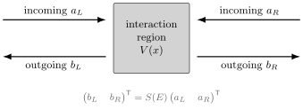
The right-moving and left-moving waves exchange their incoming or outgoing role across the interaction region. Flux normalization turns the four asymptotic coefficients into a two-channel map $\mathbf b=S\mathbf a$.

Reflection and Transmission Amplitudes

For incidence from the left, choose unit raw incoming amplitude:

$$\begin{aligned} \psi_L(x) &\sim e^{ik_Lx} + r_L e^{-ik_Lx}, &&x\to-\infty, \\ \psi_L(x) &\sim t_L e^{ik_Rx}, &&x\to+\infty. \end{aligned}$$

For incidence from the right,

$$\begin{aligned} \psi_R(x) &\sim t_R e^{-ik_Lx}, &&x\to-\infty, \\ \psi_R(x) &\sim e^{-ik_Rx} + r_R e^{ik_Rx}, &&x\to+\infty. \end{aligned}$$

Introduce flux-normalized transmission amplitudes

$$\tau_L = \sqrt{\frac{v_R}{v_L}}\,t_L, \qquad \tau_R = \sqrt{\frac{v_L}{v_R}}\,t_R.$$

In the left/right incoming basis,

$$S(E) = \begin{pmatrix} r_L & \tau_R\\ \tau_L & r_R \end{pmatrix}.$$

The observable probabilities are

$$\begin{aligned} R_L&=|r_L|^2, & T_L&=|\tau_L|^2 = \frac{v_R}{v_L}|t_L|^2, \\ R_R&=|r_R|^2, & T_R&=|\tau_R|^2 = \frac{v_L}{v_R}|t_R|^2. \end{aligned}$$

When $V_L=V_R$, the velocities agree and $\tau_{L,R}=t_{L,R}$. The familiar rule $T=|t|^2$ is therefore a special equal-velocity case, not the fundamental definition.

Unitarity and Reciprocity

For a real conservative potential with both asymptotic channels included,

$$S^\dagger S=I.$$

The two column norms give

$$|r_L|^2+|\tau_L|^2=1, \qquad |r_R|^2+|\tau_R|^2=1.$$

The columns must also be orthogonal:

$$r_L^*\tau_R + \tau_L^*r_R =0.$$

Thus unitarity constrains phases as well as probabilities. Checking only $R+T=1$ does not test the full matrix.

For spinless time-reversal-invariant scattering, channel phases can be chosen so that

$$S=S^{\mathsf T}.$$

Hence

$$\tau_L=\tau_R.$$

When the asymptotic velocities are equal, this becomes $t_L=t_R$. An asymmetric real potential can still have different reflection amplitudes $r_L$ and $r_R$, although unitarity and reciprocity constrain their magnitudes and relative phases. If the potential also has parity symmetry, then

$$r_L=r_R.$$

A complex optical potential can absorb or amplify flux, so the reduced two-channel matrix is then nonunitary. Additional physical channels can produce the same apparent deficit if they have simply been omitted.

The Transfer Matrix

The scattering matrix groups amplitudes by incoming versus outgoing status. The transfer matrix instead relates coefficients on opposite sides:

$$\begin{pmatrix} A_R^+\\ A_R^- \end{pmatrix} = M(E) \begin{pmatrix} A_L^+\\ A_L^- \end{pmatrix}.$$

Write

$$M = \begin{pmatrix} M_{11}&M_{12}\\ M_{21}&M_{22} \end{pmatrix}.$$

This convention is valuable because interfaces and propagation regions compose in spatial order. If a structure consists of successive elements,

$$M_{\mathrm{total}} = M_NM_{N-1}\cdots M_2M_1.$$

For left incidence,

$$\begin{pmatrix} t_L\\ 0 \end{pmatrix} = M \begin{pmatrix} 1\\ r_L \end{pmatrix},$$

which gives

$$r_L = -\frac{M_{21}}{M_{22}}, \qquad t_L = \frac{\det M}{M_{22}}.$$

For right incidence,

$$\begin{pmatrix} r_R\\ 1 \end{pmatrix} = M \begin{pmatrix} 0\\ t_R \end{pmatrix},$$

so

$$r_R = \frac{M_{12}}{M_{22}}, \qquad t_R = \frac{1}{M_{22}}.$$

For equal asymptotic velocities, the raw-amplitude scattering matrix is therefore

$$S = \frac{1}{M_{22}} \begin{pmatrix} -M_{21}&1\\ \det M&M_{12} \end{pmatrix}.$$

For the ordinary Schrödinger equation with equal asymptotic wave numbers,

$$\det M=1,$$

so $t_L=t_R$. If the asymptotic wave numbers differ, the raw transfer matrix need not have unit determinant; flux normalization restores the physically unitary channel description.

Transfer-matrix conventions differ. Some references propagate right to left or reverse the coefficient ordering, moving the relevant denominator from $M_{22}$ to $M_{11}$. The invariant check is to impose the stated boundary conditions and rederive $r$ and $t$ rather than memorizing an index.

Composition versus numerical stability

Transfer matrices compose elegantly but can be numerically ill-conditioned. An evanescent region introduces factors

$$e^{\kappa a} \quad\text{and}\quad e^{-\kappa a}.$$

For a thick barrier or long multilayer stack, the growing factor can overflow while the physical transmission is exponentially small. Stable scattering-matrix recursion, logarithmic derivatives, or rescaled propagation avoids multiplying enormous and tiny numbers in the same matrix.

Bound States as Scattering Poles

The same denominator that controls transmission also remembers the bound spectrum. Continue the amplitudes from real positive $k$ into the complex momentum plane. For equal asymptotic thresholds, a bound state has

$$k=i\kappa, \qquad \kappa>0.$$

At $x\to-\infty$, normalizability keeps only $e^{\kappa x}$; at $x\to+\infty$, it keeps only $e^{-\kappa x}$. In the traveling-wave notation, this means

$$A_L^+=0, \qquad A_R^-=0,$$

while $A_L^-$ and $A_R^+$ may be nonzero. These are outgoing-only boundary conditions after analytic continuation.

The transfer relation then becomes

$$\begin{pmatrix} A_R^+\\ 0 \end{pmatrix} = M(k) \begin{pmatrix} 0\\ A_L^- \end{pmatrix}.$$

A nontrivial solution requires

$$M_{22}(k)=0.$$

Since $t_R=1/M_{22}$, the same condition is a pole of the transmission amplitude. The direct bound-state matching equation and the scattering-pole equation are not separate facts; they are the same homogeneous boundary-value condition viewed on different parts of the complex energy surface.

Pole classification

For a short-range potential with threshold at $E=0$, the momentum-plane locations have different physical meanings.

Pole location	Interpretation	Spatial behavior
$k=i\kappa$, $\kappa>0$	bound state	decays at both infinities
$k=-i\kappa$, $\kappa>0$	virtual or antibound state	non-normalizable continuation
$\operatorname{Re}k>0$, $\operatorname{Im}k<0$	resonance	outgoing Gamow condition

For a resonance,

$$E_{\mathrm{pole}} = E_R-\frac{i}{2}\Gamma,$$

with $\Gamma>0$. Its analytically continued wave grows spatially, so it is not a Hilbert-space eigenstate; the negative imaginary energy instead encodes temporal decay.

Bound States and Scattering Poles owns the general analytic classification and sheet structure.

Delta-interaction check

For $V(x)=\lambda\delta(x)$, define

$$\gamma=\frac{m\lambda}{\hbar^2}.$$

The exact transmission amplitude is

$$t(k)=\frac{k}{k+i\gamma}.$$

If $\lambda<0$, then $\gamma<0$ and the pole lies at

$$k=i|\gamma|,$$

the positive imaginary axis. It reproduces the unique attractive-delta bound state. The complete matching derivation belongs at Scattering from a Delta Potential; Delta Potential Scattering audits the lead-channel swap, reduced parity eigenvalues, and pole residue in one fixed convention.

Resonant Tunneling as Repeated Scattering

Consider two barriers separated by a classically allowed region of length $L$ and wave number $k$. Let $t_1$ transmit through the first barrier from the left, $t_2$ transmit through the second, $r_1'$ reflect from the first barrier as seen from inside the middle region, and $r_2$ reflect from the second barrier as seen from inside.

The transmitted amplitude is a coherent sum over all round trips:

$$\begin{aligned} t_{\mathrm{tot}} ={}& t_1t_2e^{ikL} \sum_{n=0}^{\infty} \left( r_1'r_2e^{2ikL} \right)^n \\ ={}& \frac{ t_1t_2e^{ikL} }{ 1-r_1'r_2e^{2ikL} }. \end{aligned}$$

The $n=0$ term is the direct path through both barriers; terms with $n\ge1$ include one or more round trips. What matters is that the amplitudes form a geometric series whose denominator is produced by repeated coherent reflection.

A resonance occurs when the round-trip phase nearly satisfies

$$2kL + \arg(r_1'r_2) \approx 2\pi n,$$

and $|r_1'r_2|$ is close to one. The wave then builds up between the barriers like a leaky standing wave. High transmission does not mean that either barrier has ceased to tunnel; it means the full structure has arranged destructive interference in reflection and constructive interference in transmission.

Near an isolated resonance, a common probability form is

$$\begin{aligned} T(E) &\approx \frac{ \Gamma_L\Gamma_R }{ (E-E_R)^2+\Gamma^2/4 }, \\ \Gamma &= \Gamma_L+\Gamma_R. \end{aligned}$$

At $E=E_R$,

$$T(E_R) \approx \frac{ 4\Gamma_L\Gamma_R }{ (\Gamma_L+\Gamma_R)^2 }.$$

A symmetric lossless structure can reach unit transmission. Unequal leakage rates lower the peak. Resonant Transmission owns the double-barrier calculation, while Breit–Wigner Form owns the general isolated-pole parameterization and its limits.

Parity Channels for a Symmetric Potential

If

$$V(x)=V(-x)$$

and the asymptotic velocities agree, then

$$S = \begin{pmatrix} r&t\\ t&r \end{pmatrix}.$$

Its eigenvectors are the even and odd incoming combinations,

$$\frac{1}{\sqrt2} \begin{pmatrix} 1\\ 1 \end{pmatrix}, \qquad \frac{1}{\sqrt2} \begin{pmatrix} 1\\ -1 \end{pmatrix},$$

with eigenvalues

$$S_{\mathrm e}=r+t, \qquad S_{\mathrm o}=r-t.$$

Unitarity gives $|S_{\mathrm e}|=|S_{\mathrm o}|=1$. These eigenvalues can be described by parity phase shifts. There is a convention subtlety: in the left/right channel basis, the free-particle matrix is

$$S_{\mathrm{free}} = \begin{pmatrix} 0&1\\ 1&0 \end{pmatrix},$$

whose even and odd eigenvalues are $+1$ and $-1$. Some phase-shift conventions absorb the odd-channel minus sign so both free phase shifts vanish. Apparent sign disagreements should be traced to this free-channel convention before comparing formulas.

WKB Comparison

For a smooth barrier with turning points $x_1$ and $x_2$, define the forbidden-region action

$$K(E) = \int_{x_1}^{x_2} \sqrt{2m\left[V(x)-E\right]} \,dx.$$

The leading WKB transmission probability is

$$T_{\mathrm{WKB}} \approx e^{-2K(E)/\hbar}.$$

This formula captures the dominant suppression when $K/\hbar\gg1$. It does not by itself provide the complete complex amplitude needed for coherent composition.

Method	Main object	Strength	Main limitation
direct matching	wavefunction coefficients	exact for solvable profiles	becomes cumbersome for many regions
transfer matrix	spatial coefficient map $M$	exact composition for layered models	evanescent factors can be ill-conditioned
scattering matrix	incoming-to-outgoing map $S$	unitary and numerically stable in open channels	does not compose by naive multiplication in space
leading WKB	action $K(E)$	exposes exponential scale for smooth barriers	loses important prefactors and phases

Why probabilities cannot be multiplied coherently

For two separated barriers, multiplying the one-barrier probabilities,

$$T_{\mathrm{naive}}=T_1T_2,$$

discards the phases of all paths that bounce between them. It therefore cannot produce resonant transmission. A semiclassical treatment can recover resonances only if it keeps complex reflection amplitudes, propagation phases, and the repeated-round-trip denominator.

The WKB barrier action still has an important role near a narrow resonance. It estimates the exponentially small leakage through each barrier and therefore the partial widths $\Gamma_L$ and $\Gamma_R$. The phase accumulated in the intermediate allowed region determines the approximate resonance energy.

Leading WKB also becomes unreliable near a barrier top, at coalescing turning points, for abrupt discontinuities without separate matching, and whenever $K/\hbar$ is not large. Barrier Penetration and Tunneling owns the action formula and connection-rule caveats.

Stationary States and Wave Packets

The $S(E)$ matrix is defined at a sharp energy, but a physical incoming particle is a packet. For a left-incident momentum envelope $g(k)$, the late-time reflected and transmitted probabilities are, for equal asymptotic thresholds,

$$P_R = \int_0^\infty dk\, |g(k)|^2|r_L(k)|^2,$$

and

$$P_T = \int_0^\infty dk\, |g(k)|^2|t_L(k)|^2.$$

If the packet is narrow around $k_0$, then $P_R\approx R(k_0)$ and $P_T\approx T(k_0)$. A broad packet samples energy-dependent magnitudes and phases, so it can distort, split, or acquire a delay.

The phase of a scattering amplitude matters even when a stationary transmission probability does not show it. Near a resonance, rapid phase variation is associated with temporary probability storage in the interaction region. Wave Packets and Scattering owns the time-dependent construction.

Practical Workflow

1. State the asymptotic potentials and determine which left and right channels are open.
2. Fix whether amplitudes are raw wave coefficients or flux normalized.
3. Define the ordering and propagation direction of the transfer matrix before multiplying layers.
4. Extract both left- and right-incidence amplitudes as a convention check.
5. Verify $S^\dagger S=I$ for a real conservative model.
6. Test reciprocity and, when applicable, parity symmetry.
7. Locate bound or resonance states from outgoing-only boundary conditions or zeros of the transfer denominator.
8. Use WKB only in a controlled smooth-barrier regime, retaining phases for multibarrier interference.
9. Fold stationary amplitudes with the incident packet or experimental energy distribution.

Common Mistakes

• Calling $R$ or $T$ a three-dimensional cross section; they are dimensionless channel probabilities.
• Treating the $+$ and $-$ traveling-wave labels as incoming and outgoing on both sides.
• Writing $T=|t|^2$ when the asymptotic velocities differ.
• Comparing transfer-matrix entries across sources without matching coefficient ordering and propagation direction.
• Multiplying transfer matrices through thick evanescent regions without checking numerical conditioning.
• Checking only $R+T=1$ and ignoring the phase orthogonality required by full $S$-matrix unitarity.
• Assuming asymmetric real potentials have identical reflection amplitudes from both sides.
• Identifying every transmission maximum as a resonance without checking phase motion, internal buildup, or pole structure.
• Treating a resonance pole state as a normalizable bound state.
• Multiplying single-barrier transmission probabilities and thereby erasing resonant interference.
• Using the leading WKB exponent near a barrier top or as a substitute for an exact phase-sensitive amplitude.

Exercises

1. Build the flux-normalized S-matrix

Starting from raw left- and right-incidence amplitudes $r_L,t_L,r_R,t_R$ with asymptotic velocities $v_L$ and $v_R$, construct the flux-normalized scattering matrix and identify the four channel probabilities.

Solution

The incoming flux vector is

$$\mathbf a = \begin{pmatrix} \sqrt{v_L}A_L^+\\ \sqrt{v_R}A_R^- \end{pmatrix},$$

and the outgoing flux vector is

$$\mathbf b = \begin{pmatrix} \sqrt{v_L}A_L^-\\ \sqrt{v_R}A_R^+ \end{pmatrix}.$$

Therefore

$$S = \begin{pmatrix} r_L & \sqrt{v_L/v_R}\,t_R \\ \sqrt{v_R/v_L}\,t_L & r_R \end{pmatrix}.$$

The probabilities are

$$\begin{aligned} R_L&=|r_L|^2, & T_L&=\frac{v_R}{v_L}|t_L|^2, \\ R_R&=|r_R|^2, & T_R&=\frac{v_L}{v_R}|t_R|^2. \end{aligned}$$

For a unitary two-channel problem, $R_L+T_L=R_R+T_R=1$.

2. Convert a transfer matrix to scattering amplitudes

Let

$$\begin{pmatrix} A_R^+\\ A_R^- \end{pmatrix} = \begin{pmatrix} M_{11}&M_{12}\\ M_{21}&M_{22} \end{pmatrix} \begin{pmatrix} A_L^+\\ A_L^- \end{pmatrix}.$$

Derive $r_L,t_L,r_R,t_R$.

Solution

For left incidence,

$$\begin{pmatrix} t_L\\ 0 \end{pmatrix} = M \begin{pmatrix} 1\\ r_L \end{pmatrix}.$$

The lower row gives

$$r_L=-\frac{M_{21}}{M_{22}},$$

and substitution into the upper row gives

$$t_L=\frac{\det M}{M_{22}}.$$

For right incidence,

$$\begin{pmatrix} r_R\\ 1 \end{pmatrix} = M \begin{pmatrix} 0\\ t_R \end{pmatrix}.$$

Hence

$$t_R=\frac{1}{M_{22}}, \qquad r_R=\frac{M_{12}}{M_{22}}.$$

If $\det M=1$, the two transmission amplitudes agree.

3. Recover the attractive-delta bound state from a pole

For

$$t(k)=\frac{k}{k+i\gamma}, \qquad \gamma=\frac{m\lambda}{\hbar^2},$$

locate the pole for $\lambda<0$ and find its energy.

Solution

For an attractive interaction, $\gamma=-|\gamma|$. The denominator vanishes at

$$k+i\gamma = k-i|\gamma| =0,$$

so

$$k=i|\gamma|.$$

This lies on the positive imaginary axis and gives

$$E = \frac{\hbar^2k^2}{2m} = -\frac{\hbar^2\gamma^2}{2m} = -\frac{m\lambda^2}{2\hbar^2}.$$

The pole energy is exactly the bound-state eigenvalue obtained by solving the normalizable boundary-value problem directly.

4. Unitarity constrains phases

For equal asymptotic velocities, take

$$S = \begin{pmatrix} r_L&t\\ t&r_R \end{pmatrix}.$$

Derive the conditions imposed by unitarity and explain why $R+T=1$ is not the whole statement.

Solution

The diagonal elements of $S^\dagger S=I$ give

$$|r_L|^2+|t|^2=1, \qquad |r_R|^2+|t|^2=1.$$

The off-diagonal element gives

$$r_L^*t+t^*r_R=0.$$

The first two relations imply $|r_L|=|r_R|$, but the third fixes a relative phase relation. Two sets of amplitudes can obey $R+T=1$ while failing to form a unitary scattering matrix if their phases violate the off-diagonal condition.

5. Sum the round trips

A wave crosses a first barrier with amplitude $t_1$, propagates through a middle region with phase $e^{ikL}$, and crosses a second barrier with amplitude $t_2$. Each complete round trip multiplies the amplitude by

$$z=r_1'r_2e^{2ikL}.$$

Sum the transmitted paths and state the resonance condition.

Solution

The direct path contributes

$$t_1t_2e^{ikL}.$$

Paths with $n$ round trips contribute an additional factor $z^n$, so

$$t_{\mathrm{tot}} = t_1t_2e^{ikL} \sum_{n=0}^{\infty}z^n = \frac{ t_1t_2e^{ikL} }{ 1-r_1'r_2e^{2ikL} },$$

provided $|z|<1$ on the physical real-energy axis. Transmission is resonantly enhanced when the denominator is small:

$$2kL+\arg(r_1'r_2) \approx 2\pi n,$$

with $|r_1'r_2|$ close to one.

6. Why the leading WKB probability misses a resonance

Explain why using

$$T_j\approx e^{-2K_j/\hbar}$$

for each of two barriers and then multiplying $T_1T_2$ cannot predict unit resonant transmission.

Solution

Each $T_j$ contains only a probability and therefore discards the complex reflection and transmission phases. A double barrier admits infinitely many paths that differ by round trips in the middle region. Those amplitudes must be added before squaring:

$$t_{\mathrm{tot}} \propto \frac{ e^{-(K_1+K_2)/\hbar} e^{i\Phi} }{ 1-r_1'r_2e^{2i\Phi} }.$$

Near a resonance, the denominator can compensate for the small numerator and produce large or unit transmission in a symmetric lossless structure. Multiplying $T_1T_2$ keeps only the direct path and cannot represent that interference. WKB can still estimate the leakage widths if its complex amplitudes and connection phases are retained.

Cross-Links

• Reflection and Transmission Coefficients
• Transfer Matrix Method
• Scattering from a Delta Potential
• Resonant Transmission
• Wave Packets and Scattering
• S-Matrix
• Bound States and Scattering Poles
• Delta Potential Scattering
• Resonances
• Breit–Wigner Form
• Barrier Penetration and Tunneling

References

• J. R. Taylor, Scattering Theory: The Quantum Theory of Nonrelativistic Collisions, Wiley, 1972.
• R. G. Newton, Scattering Theory of Waves and Particles, 2nd ed., Springer, 1982.
• L. D. Landau and E. M. Lifshitz, Quantum Mechanics: Non-Relativistic Theory, 3rd ed., Pergamon, 1977.
• D. J. Griffiths and D. F. Schroeter, Introduction to Quantum Mechanics, 3rd ed., Cambridge University Press, 2018.
• M. Razavy, Quantum Theory of Tunneling, World Scientific, 2003.
• S. Datta, Electronic Transport in Mesoscopic Systems, Cambridge University Press, 1995.
• E. H. Hauge and J. A. Støvneng, “Tunneling times: a critical review,” Reviews of Modern Physics 61, 917–936 (1989), doi:10.1103/RevModPhys.61.917.