Delta Potential Scattering

The one-dimensional delta interaction is exactly solvable, but it is not merely an elementary boundary-matching exercise. In one compact model it displays:

• reflection and transmission with nontrivial phases;
• a two-channel unitary scattering matrix;
• parity-channel diagonalization;
• analytic continuation in complex momentum;
• a bound-state pole for attraction and a non-normalizable lower-axis pole for repulsion.

This worked problem makes those structures explicit and keeps the channel convention visible. Scattering from a Delta Potential remains the canonical home for the elementary matching derivation and narrow-barrier limit. One-Dimensional Scattering Revisited owns the general channel, transfer-matrix, and pole framework. Here one exact model is carried through the full audit.

Problem Statement

Consider

$$H = -\frac{\hbar^2}{2m} \frac{d^2}{dx^2} + \lambda\delta(x),$$

with real $\lambda$. Define

$$\gamma \equiv \frac{m\lambda}{\hbar^2}.$$

The parameter $\gamma$ has dimensions of inverse length:

• $\gamma\gt0$ is a repulsive point barrier;
• $\gamma\lt0$ is an attractive point well.

For an incident energy $E\gt0$, let

$$k = \frac{\sqrt{2mE}}{\hbar} \gt0.$$

The goals are to derive the exact amplitudes, assemble the two-lead $S$ matrix, identify its parity phases, continue it to complex $k$, and recover the attractive bound state from its pole.

Matching Data

Away from the origin the particle is free. Integrating the Schrödinger equation across $x=0$ gives

$$\psi(0^+)=\psi(0^-),$$

and

$$\psi'(0^+)-\psi'(0^-) = 2\gamma\psi(0).$$

The wavefunction is continuous; its derivative is not. These two relations contain the entire point interaction.

For incidence from the left, use

$$\psi_L(x) = \begin{cases} e^{ikx} + r(k)e^{-ikx}, & x\lt0, \\ t(k)e^{ikx}, & x\gt0. \end{cases}$$

Continuity gives

$$1+r=t.$$

The derivative jump gives

$$ik\,t - ik(1-r) = 2\gamma t.$$

Eliminating $t$,

$$ik\,r = \gamma(1+r).$$

Therefore

$$\begin{aligned} r(k) &= \frac{ -i\gamma }{ k+i\gamma }, \\ t(k) &= \frac{ k }{ k+i\gamma }. \end{aligned}$$

The identity

$$t-r=1$$

is a useful algebraic check. It is also the statement that the odd parity channel, which vanishes at the origin, is unaffected by the interaction after the free-channel convention is removed.

Flux Check

The asymptotic wave number is $k$ on both sides, so the current ratios are

$$R=\lvert r\rvert^2, \qquad T=\lvert t\rvert^2.$$

For real $k$ and $\gamma$,

$$\begin{aligned} R &= \frac{ \gamma^2 }{ k^2+\gamma^2 }, \\ T &= \frac{ k^2 }{ k^2+\gamma^2 }. \end{aligned}$$

Hence

$$R+T=1.$$

The stronger amplitude-level relation is

$$r^*t+t^*r=0.$$

Thus the reflected and transmitted amplitudes have the relative phase required by unitarity, not merely probabilities that happen to add to one.

A Concrete Sign Audit

Write

$$\kappa=\lvert\gamma\rvert,$$

and choose

$$k=2\kappa.$$

For the repulsive interaction, $\gamma=+\kappa$:

$$\begin{aligned} t_+ &= 0.8-0.4i, \\ r_+ &= -0.2-0.4i. \end{aligned}$$

For the attractive interaction, $\gamma=-\kappa$:

$$\begin{aligned} t_- &= 0.8+0.4i, \\ r_- &= -0.2+0.4i. \end{aligned}$$

Both signs give

$$T=0.8, \qquad R=0.2,$$

but their amplitudes are complex conjugates. Equal probabilities do not mean equal scattering data.

The transmission phases are

$$\arg t_\pm = \mp \arctan\left(\frac12\right) = \mp0.463648\ldots.$$

That sign can be observed through interference with a reference path or through composition with a second scatterer.

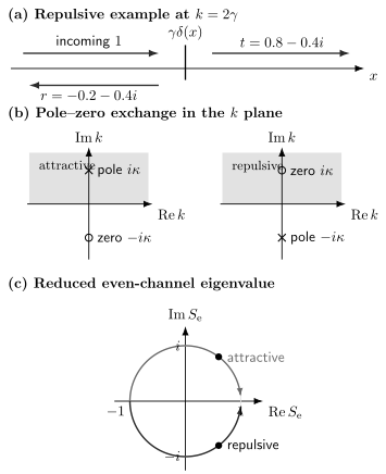
Top: the repulsive example at $k=2\gamma$ has $t=0.8-0.4i$ and $r=-0.2-0.4i$. Middle: changing the sign of the interaction exchanges the pole and zero across the real $k$ axis; only the attractive upper-axis pole is a normalizable bound state. Bottom: the reduced even-channel eigenvalue stays on the unit circle, traversing conjugate arcs for equal-magnitude attraction and repulsion.

The Two-Lead Scattering Matrix

At fixed $k$, define incoming amplitudes by

$$\mathbf a_{\mathrm{in}} = \begin{pmatrix} a_L\\ a_R \end{pmatrix},$$

where $a_L$ enters from $x=-\infty$ and $a_R$ enters from $x=+\infty$. Define outgoing amplitudes by

$$\mathbf b_{\mathrm{out}} = \begin{pmatrix} b_L\\ b_R \end{pmatrix},$$

where $b_L$ leaves toward $x=-\infty$ and $b_R$ leaves toward $x=+\infty$.

Parity and time-reversal symmetry give

$$\mathbf b_{\mathrm{out}} = S_{\mathrm{lead}} \mathbf a_{\mathrm{in}},$$

with

$$S_{\mathrm{lead}}(k) = \begin{pmatrix} r&t\\ t&r \end{pmatrix}.$$

For zero interaction,

$$S_{\mathrm{lead}}^{(0)} = \begin{pmatrix} 0&1\\ 1&0 \end{pmatrix}.$$

This is not the identity: a freely incoming wave from the left exits through the right lead. The lead basis labels spatial sides rather than propagation directions.

Unitarity

Direct multiplication gives

$$S_{\mathrm{lead}}^\dagger S_{\mathrm{lead}} = I$$

because

$$\lvert r\rvert^2+\lvert t\rvert^2=1, \qquad r^*t+t^*r=0.$$

The matrix is also symmetric,

$$S_{\mathrm{lead}}^T=S_{\mathrm{lead}},$$

as required by reciprocity for this real, time-reversal-invariant problem.

Remove the Free Lead Exchange

To compare phases with a convention in which free scattering is the identity, define

$$S_{\mathrm{red}} \equiv S_{\mathrm{lead}}^{(0)} S_{\mathrm{lead}}.$$

Since both matrices are symmetric under left–right exchange,

$$S_{\mathrm{red}} = \begin{pmatrix} t&r\\ r&t \end{pmatrix}.$$

Now

$$\lambda=0 \quad\Longrightarrow\quad S_{\mathrm{red}}=I.$$

This reduced matrix differs from the lead matrix only by a fixed free-channel convention. Probabilities are unchanged, but its eigenphases can be compared directly with the usual statement that a free phase shift vanishes.

Parity Channels

The normalized even and odd channel vectors are

$$\mathbf v_{\mathrm e} = \frac1{\sqrt2} \begin{pmatrix} 1\\ 1 \end{pmatrix}, \qquad \mathbf v_{\mathrm o} = \frac1{\sqrt2} \begin{pmatrix} 1\\ -1 \end{pmatrix}.$$

They diagonalize $S_{\mathrm{red}}$:

$$\begin{aligned} S_{\mathrm e}(k) &= t+r = \frac{ k-i\gamma }{ k+i\gamma }, \\ S_{\mathrm o}(k) &= t-r = 1. \end{aligned}$$

The delta interaction changes only the even channel. For real $k$,

$$\lvert S_{\mathrm e}\rvert = \lvert S_{\mathrm o}\rvert = 1.$$

Write

$$S_{\mathrm e}=e^{2i\delta_{\mathrm e}}, \qquad S_{\mathrm o}=e^{2i\delta_{\mathrm o}}.$$

A continuous branch at positive $k$ can be chosen as

$$\delta_{\mathrm e}(k) = -\arctan \left( \frac{\gamma}{k} \right), \qquad \delta_{\mathrm o}(k)=0,$$

modulo integer multiples of $\pi$. At $k=2\kappa$,

$$S_{\mathrm e}^{(\pm)} = 0.6\mp0.8i,$$

where the upper sign denotes repulsion. These points lie on conjugate halves of the unit circle.

In the un-reduced lead matrix, the odd eigenvalue is $r-t=-1$. That minus sign is already present for a free particle and should not be mistaken for an interaction-induced phase.

Analytic Continuation in Momentum

For complex $k$, the amplitudes are meromorphic:

$$t(k) = \frac{k}{k+i\gamma}, \qquad r(k) = \frac{-i\gamma}{k+i\gamma}.$$

The interacting parity eigenvalue is

$$S_{\mathrm e}(k) = \frac{k-i\gamma}{k+i\gamma}.$$

Its pole is at

$$k_{\mathrm p} = -i\gamma,$$

and its zero is at the reflected point

$$k_{\mathrm z} = i\gamma.$$

For a real potential, this pole–zero pairing is the analytic continuation of real-axis unitarity.

The $k$ plane is especially convenient because

$$E = \frac{\hbar^2k^2}{2m}$$

turns the energy threshold $E=0$ into the meeting point of two momentum sheets. A pole on the positive imaginary $k$ axis has negative real energy and a decaying spatial wavefunction.

Attractive Pole and Bound State

Let

$$\gamma=-\kappa, \qquad \kappa\gt0.$$

Then

$$t(k) = \frac{k}{k-i\kappa},$$

and the pole is at

$$k=i\kappa.$$

At this value, the outgoing wave on each side becomes a decaying exponential:

$$\psi_{\mathrm b}(x) = C e^{-\kappa\lvert x\rvert}.$$

The jump condition gives

$$-2\kappa C = 2\gamma C,$$

which is satisfied precisely because $\gamma=-\kappa$.

Normalization fixes

$$1 = \int_{-\infty}^{\infty} \lvert\psi_{\mathrm b}(x)\rvert^2\,dx = \frac{\lvert C\rvert^2}{\kappa},$$

so one may choose

$$C=\sqrt\kappa.$$

The pole energy is

$$\begin{aligned} E_{\mathrm b} &= \frac{\hbar^2(i\kappa)^2}{2m} \\ &= -\frac{\hbar^2\kappa^2}{2m} \\ &= -\frac{m\lambda^2}{2\hbar^2}. \end{aligned}$$

This is the unique bound state of the attractive delta potential.

Pole Residue and Tail Normalization

Near $k=i\kappa$,

$$\begin{aligned} t(k) &= \frac{k}{k-i\kappa}, \\ r(k) &= \frac{i\kappa}{k-i\kappa}. \end{aligned}$$

Their residues are

$$\operatorname*{Res}_{k=i\kappa}t = i\kappa, \qquad \operatorname*{Res}_{k=i\kappa}r = i\kappa.$$

Consequently,

$$\operatorname*{Res}_{k=i\kappa} S_{\mathrm e}(k) = 2i\kappa.$$

Since the normalized bound-state tail has $C^2=\kappa$, this model obeys

$$\operatorname*{Res}_{k=i\kappa} S_{\mathrm e}(k) = 2iC^2.$$

The exact numerical factor depends on channel and state normalization conventions, but the structural lesson is general: a bound-state pole carries information not only about its energy but also about the normalization of its asymptotic tail.

Repulsive Lower-Axis Pole

For $\gamma=+\kappa$, the pole is instead

$$k=-i\kappa.$$

The corresponding outgoing continuation grows as

$$e^{+\kappa\lvert x\rvert}$$

and is not square-integrable. It is a lower-imaginary-axis virtual or antibound continuation, not an eigenvector of the self-adjoint Hamiltonian.

The repulsive interaction has a zero at $k=i\kappa$, but an $S$-matrix zero is not a bound state. Poles and zeros exchange when the sign of $\lambda$ is reversed:

$$S_{\mathrm e}(k;-\gamma) = \frac{1}{ S_{\mathrm e}(k;\gamma) }.$$

This identity explains why the real-axis phases are conjugate while the probabilities agree.

No Resonance Pole

A resonance in one-dimensional short-range scattering would appear at complex $k$ with

$$\operatorname{Re}k\ne0, \qquad \operatorname{Im}k\lt0.$$

The single delta interaction has only the purely imaginary pole $k=-i\gamma$. It can support one bound state when attractive, but it has no finite-width quasi-bound region and therefore no off-axis resonance pair.

Two separated point interactions are different: propagation between them supplies an additional phase and can create resonance structure. That model belongs to Double Delta Potential.

High-Energy Expansion and Born Check

For

$$\frac{\lvert\gamma\rvert}{k}\ll1,$$

the exact amplitudes expand as

$$\begin{aligned} t(k) &= 1 - i\frac{\gamma}{k} - \frac{\gamma^2}{k^2} + O\left( \frac{\gamma^3}{k^3} \right), \\ r(k) &= -i\frac{\gamma}{k} - \frac{\gamma^2}{k^2} + O\left( \frac{\gamma^3}{k^3} \right). \end{aligned}$$

The leading reflected amplitude,

$$r^{(1)} = -i\frac{\gamma}{k},$$

is the one-dimensional first-Born result for a contact interaction in this normalization. The exact denominator $1+i\gamma/k$ resums repeated interactions at the point.

At low energy, $\lvert\gamma\rvert/k\gg1$, this expansion fails even if $\lvert\lambda\rvert$ is numerically small in dimensional units. The correct dimensionless control parameter is $\lvert\gamma\rvert/k$, not $\lambda$ by itself.

Limiting Checks

Zero coupling

As $\gamma\to0$,

$$t\to1, \qquad r\to0, \qquad S_{\mathrm{red}}\to I.$$

High energy

As $k\to\infty$ at fixed $\gamma$,

$$T\to1, \qquad R\sim\frac{\gamma^2}{k^2}.$$

Low energy

As $k\to0^+$ at nonzero fixed $\gamma$,

$$t\to0, \qquad r\to-1.$$

The point interaction becomes perfectly reflecting at threshold. The approach to that limit still carries sign-dependent phase information.

Sign reversal

For real $k$,

$$\begin{aligned} t(k;-\gamma)&=t(k;\gamma)^*, \\ r(k;-\gamma)&=r(k;\gamma)^*. \end{aligned}$$

This proves equality of $R$ and $T$ and conjugacy of the full amplitudes.

Validity and Scope

The delta potential is not an approximation once it is defined as a self-adjoint point interaction with the stated matching condition. Its use as a model of a finite-range interaction is an approximation whose validity requires wavelengths long compared with the physical range and no sensitivity to omitted effective-range structure.

The formulas also assume:

• a real coupling and hence a Hermitian Hamiltonian;
• equal free thresholds and masses on both sides;
• one point interaction at the origin;
• the standard continuous-wavefunction delta interaction rather than a more general point-interaction boundary condition.

A complex $\lambda$ would model absorption or gain and destroy unitarity. A derivative-delta interaction or a general $U(2)$ point interaction can make the wavefunction itself discontinuous and has different matching data.

Common Mistakes

• Enforcing continuity of $\psi'$ instead of its delta-induced jump.
• Forgetting that $\lambda$ has dimensions of energy times length.
• Comparing $\lambda$ directly with $k$ instead of using the dimensionless ratio $\gamma/k$.
• Squaring amplitudes before checking their phases and unitarity relation.
• Writing the lead-basis free $S$ matrix as the identity without changing channel convention.
• Calling the lead odd eigenvalue $-1$ an interaction phase.
• Treating the attractive and repulsive interactions as identical because they have the same $R$ and $T$.
• Interpreting the repulsive lower-axis pole as a normalizable state.
• Calling an upper-axis zero a bound state.
• Looking for a resonance width in a model whose only pole is purely imaginary.

Exercises

1. Re-derive the amplitudes

Starting from continuity and the derivative jump, derive $r(k)$ and $t(k)$ without using the formulas above.

Solution

Continuity gives

$$t=1+r.$$

The jump condition is

$$ik\,t-ik(1-r) = 2\gamma t.$$

Substitution gives

$$2ik\,r = 2\gamma(1+r),$$

or

$$r = \frac{\gamma}{ik-\gamma} = \frac{-i\gamma}{k+i\gamma}.$$

Then

$$t=1+r = \frac{k}{k+i\gamma}.$$

2. Diagonalize both S-matrix conventions

Find the parity eigenvalues of $S_{\mathrm{lead}}$ and $S_{\mathrm{red}}$. Explain the odd-channel sign difference.

Solution

For the even vector $(1,1)^T/\sqrt2$,

$$S_{\mathrm{lead}} \mathbf v_{\mathrm e} = (r+t) \mathbf v_{\mathrm e}.$$

For the odd vector $(1,-1)^T/\sqrt2$,

$$S_{\mathrm{lead}} \mathbf v_{\mathrm o} = (r-t) \mathbf v_{\mathrm o} = -\mathbf v_{\mathrm o}.$$

Thus the lead eigenvalues are $r+t$ and $-1$. Multiplication by the free swap matrix leaves the even eigenvalue unchanged and reverses the odd one:

$$S_{\mathrm e}^{\mathrm{red}} = r+t, \qquad S_{\mathrm o}^{\mathrm{red}} = t-r = 1.$$

The lead-basis minus sign is the eigenvalue of free left–right exchange in the odd channel, not scattering from the delta interaction.

3. Verify the k = 2κ audit

For $\gamma=\pm\kappa$ and $k=2\kappa$, compute $r$, $t$, $R$, $T$, and the reduced even-channel eigenvalue.

Solution

For $\gamma=+\kappa$,

$$t = \frac2{2+i} = \frac{4-2i}{5} = 0.8-0.4i,$$

and

$$r=t-1=-0.2-0.4i.$$

For $\gamma=-\kappa$, both amplitudes are complex conjugated. In either case,

$$T=\lvert t\rvert^2=0.8, \qquad R=\lvert r\rvert^2=0.2.$$

Finally,

$$S_{\mathrm e} = t+r = 0.6\mp0.8i,$$

with the upper sign for repulsion.

4. Recover the bound state from the pole

For $\lambda\lt0$, show that the pole condition gives the normalized bound state and its energy.

Solution

Write $\gamma=-\kappa$ with $\kappa\gt0$. The denominator vanishes at

$$k=i\kappa.$$

The decaying solution is

$$\psi(x)=C e^{-\kappa\lvert x\rvert}.$$

Its derivative jump is $-2\kappa C$, equal to $2\gamma C$ because $\gamma=-\kappa$. Normalization gives

$$1 = 2\lvert C\rvert^2 \int_0^\infty e^{-2\kappa x}\,dx = \frac{\lvert C\rvert^2}{\kappa},$$

so $C=\sqrt\kappa$ up to a phase. The energy is

$$E_{\mathrm b} = -\frac{\hbar^2\kappa^2}{2m} = -\frac{m\lambda^2}{2\hbar^2}.$$

5. Relate the pole residue to the tail

Compute the residue of $S_{\mathrm e}$ at the attractive pole and express it in terms of the bound-state tail coefficient $C$.

Solution

For $\gamma=-\kappa$,

$$S_{\mathrm e}(k) = \frac{k+i\kappa}{k-i\kappa}.$$

Therefore

$$\operatorname*{Res}_{k=i\kappa} S_{\mathrm e} = \left. \left( k+i\kappa \right) \right|_{k=i\kappa} = 2i\kappa.$$

Since $C=\sqrt\kappa$,

$$\operatorname*{Res}_{k=i\kappa} S_{\mathrm e} = 2iC^2.$$

6. Identify the Born regime

Expand the exact reflected amplitude through second order in $\gamma/k$. At what energy scale is the first term reliable?

Solution

Using

$$\frac1{1+iz} = 1-iz-z^2+O(z^3),$$

with $z=\gamma/k$,

$$r = -i\frac{\gamma}{k} - \frac{\gamma^2}{k^2} + O\left( \frac{\gamma^3}{k^3} \right).$$

The first term is reliable when

$$\frac{\lvert\gamma\rvert}{k}\ll1,$$

or

$$E \gg \frac{\hbar^2\gamma^2}{2m}.$$

The same scale is the magnitude of the attractive bound-state energy, which is a useful independent dimensional check.

Cross-Links

• Scattering from a Delta Potential owns the canonical matching calculation and narrow-barrier limit.
• Delta-Function Potential derives the attractive bound state directly.
• One-Dimensional Scattering Revisited develops the general two-lead, transfer-matrix, parity, and pole framework.
• S-Matrix gives the operator-level scattering definition and unitarity structure.
• Bound States and Scattering Poles classifies bound, virtual, and resonance poles.
• Complex Analysis Essentials reviews residues and analytic continuation.

References

1. S. Albeverio, F. Gesztesy, R. Høegh-Krohn, and H. Holden, Solvable Models in Quantum Mechanics, 2nd ed., AMS Chelsea (2005).
2. J. R. Taylor, Scattering Theory: The Quantum Theory of Nonrelativistic Collisions, Dover (2006).
3. R. G. Newton, Scattering Theory of Waves and Particles, 2nd ed., Dover (2002).
4. C. J. Joachain, Quantum Collision Theory, 3rd ed., North-Holland (1983).
5. D. J. Griffiths and D. F. Schroeter, Introduction to Quantum Mechanics, 3rd ed., Cambridge University Press (2018).