Yukawa Potential in the Born Approximation

The Yukawa potential is the screened Coulomb form

$$V(r) = g\frac{e^{-\mu r}}{r}, \qquad \mu>0.$$

Its first Born amplitude is elementary, but the result carries several lessons at once: screening regulates the Coulomb forward singularity, the angular distribution becomes forward-peaked when the wavelength is short compared with the screening length, and the same momentum-space denominator appears in the static limit of massive-particle exchange.

This page works out those statements quantitatively. The First Born Approximation remains the canonical home for the general derivation from the Lippmann–Schwinger equation.

Problem Statement and Conventions

Consider elastic scattering from

$$H = -\frac{\hbar^2}{2m}\nabla^2 + g\frac{e^{-\mu r}}{r}.$$

Here:

• $m$ is the projectile mass for a fixed scattering center, or the reduced mass in the two-body relative-coordinate problem;
• $g$ has dimensions of energy times length;
• $g>0$ is repulsive and $g<0$ is attractive;
• $\mu^{-1}$ is the screening length;
• $E=\hbar^2k^2/(2m)$ is the incident relative kinetic energy.

The incoming and outgoing wave vectors have equal magnitude $k$. Their momentum transfer is

$$\mathbf q = \mathbf k'-\mathbf k, \qquad q = 2k\sin\frac{\theta}{2}.$$

The observables to be calculated are the differential cross section, total cross section, momentum-transfer cross section, threshold scattering length, and first-order partial-wave phase shifts.

Method Choice

With the convention used throughout this volume, the first Born amplitude is

$$f_{\mathrm B}(\mathbf q) = -\frac{m}{2\pi\hbar^2} \widetilde V(\mathbf q),$$

where

$$\widetilde V(\mathbf q) = \int d^3r\, e^{-i\mathbf q\cdot\mathbf r}V(r).$$

The method is attractive here because the Yukawa transform is analytic. That convenience is not a validity proof. The potential is singular as $r\to0$, and an attractive Yukawa interaction can develop a near-threshold bound state when its dimensionless strength becomes order unity. Both facts must be checked after the transform is evaluated.

Dimensionless Variables

Introduce

$$x = \frac{k}{\mu}, \qquad y = \frac{q}{\mu} = 2x\sin\frac{\theta}{2},$$

and the signed coupling

$$\lambda = \frac{2mg}{\hbar^2\mu}.$$

The parameter $x$ compares the screening length with the reduced wavelength. The magnitude $|\lambda|$ compares the interaction with the kinetic localization scale associated with the range $\mu^{-1}$.

The sign of $\lambda$ distinguishes repulsion from attraction. The leading Born cross sections depend on $\lambda^2$, but the amplitude, phase shifts, scattering length, higher Born terms, and bound-state content retain the sign.

Fourier Transform

For a central potential,

$$\widetilde V(q) = 4\pi \int_0^\infty dr\, r^2V(r) \frac{\sin(qr)}{qr}.$$

Substituting the Yukawa form gives

$$\begin{aligned} \widetilde V(q) &= 4\pi g \int_0^\infty dr\, r e^{-\mu r} \frac{\sin(qr)}{qr} \\ &= \frac{4\pi g}{q} \int_0^\infty dr\, e^{-\mu r}\sin(qr). \end{aligned}$$

The remaining integral is

$$\int_0^\infty dr\, e^{-\mu r}\sin(qr) = \frac{q}{q^2+\mu^2}.$$

Therefore

$$\widetilde V(q) = \frac{4\pi g}{q^2+\mu^2}.$$

Green-function check

The same result follows from the distributional identity

$$\left( -\nabla^2+\mu^2 \right) \frac{e^{-\mu r}}{r} = 4\pi\delta^{(3)}(\mathbf r).$$

Fourier transformation turns $-\nabla^2+\mu^2$ into multiplication by $q^2+\mu^2$, so

$$\left(q^2+\mu^2\right) \int d^3r\, e^{-i\mathbf q\cdot\mathbf r} \frac{e^{-\mu r}}{r} = 4\pi.$$

This check fixes both the denominator and the factor $4\pi$.

Born Amplitude

Substituting the transform into the Born formula yields

$$f_{\mathrm B}(q) = -\frac{2mg}{\hbar^2} \frac{1}{q^2+\mu^2}.$$

In dimensionless form,

$$\mu f_{\mathrm B}(\theta) = -\frac{\lambda} {1+4x^2\sin^2(\theta/2)}.$$

Several features are immediate:

• the amplitude has dimensions of length;
• screening keeps $f_{\mathrm B}(0)$ finite;
• repulsion and attraction give opposite leading amplitudes;
• momentum transfers $q\gg\mu$ are suppressed algebraically as $q^{-2}$.

The algebraic tail differs from the exponential momentum-space suppression of a smooth Gaussian potential. The difference traces back to the Yukawa potential’s $1/r$ singularity at the origin.

Differential Cross Section

The elastic differential cross section is

$$\frac{d\sigma_{\mathrm B}}{d\Omega} = \left|f_{\mathrm B}(\theta)\right|^2.$$

Thus

$$\frac{d\sigma_{\mathrm B}}{d\Omega} = \frac{4m^2g^2}{\hbar^4} \frac{1} {\left[ \mu^2+4k^2\sin^2(\theta/2) \right]^2}.$$

Equivalently,

$$\mu^2 \frac{d\sigma_{\mathrm B}}{d\Omega} = \frac{\lambda^2} {\left[ 1+4x^2\sin^2(\theta/2) \right]^2}.$$

The forward value is independent of $k$ at fixed $g$ and $\mu$:

$$\left. \frac{d\sigma_{\mathrm B}}{d\Omega} \right|_{\theta=0} = \frac{4m^2g^2}{\hbar^4\mu^4} = \frac{\lambda^2}{\mu^2}.$$

The backward-to-forward ratio is

$$\frac{ \left.d\sigma/d\Omega\right|_{\theta=\pi} }{ \left.d\sigma/d\Omega\right|_{\theta=0} } = \frac{1}{\left(1+4x^2\right)^2}.$$

At $x\ll1$, the denominator changes little over the sphere and the scattering is approximately isotropic. At $x\gg1$, appreciable scattering is confined to angles of order

$$\theta \sim \frac{\mu}{k} = \frac{1}{x}.$$

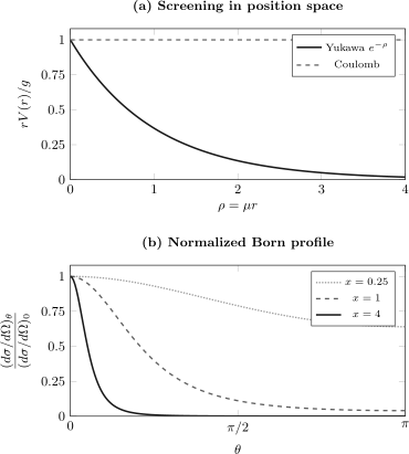
Multiplying the potential by $r/g$ isolates the screening factor $e^{-\mu r}$ from the Coulomb singularity. In momentum space, the normalized Born profile is $[1+4x^2\sin^2(\theta/2)]^{-2}$: it is nearly isotropic for $x=k/\mu\ll1$ and becomes a forward cone for $x\gg1$.

Total Cross Section

Set $u=\cos\theta$. Then

$$\sigma_{\mathrm B} = 2\pi\frac{\lambda^2}{\mu^2} \int_{-1}^{1} \frac{du} {\left[ 1+2x^2(1-u) \right]^2}.$$

The angular integral is

$$\int_{-1}^{1} \frac{du} {\left[ 1+2x^2(1-u) \right]^2} = \frac{2}{1+4x^2}.$$

Hence

$$\sigma_{\mathrm B} = \frac{4\pi\lambda^2} {\mu^2\left(1+4x^2\right)}.$$

In dimensional variables,

$$\sigma_{\mathrm B} = \frac{16\pi m^2g^2} {\hbar^4\mu^2\left(\mu^2+4k^2\right)}.$$

Low-energy limit

For $x\ll1$,

$$\sigma_{\mathrm B} = \frac{4\pi\lambda^2}{\mu^2} \left[ 1-4x^2+O(x^4) \right].$$

This is the isotropic $s$-wave limit.

High-energy limit

For $x\gg1$,

$$\sigma_{\mathrm B} \sim \frac{\pi\lambda^2}{k^2}.$$

The forward differential cross section remains finite, but the angular cone narrows as $\mu/k$. Its shrinking solid angle makes the total cross section fall as $k^{-2}$.

Momentum-Transfer Cross Section

For a strongly forward-peaked distribution, the total cross section counts many events that barely change the longitudinal momentum. Transport applications therefore use

$$\sigma_{\mathrm{tr}} = \int d\Omega\, \left(1-\cos\theta\right) \frac{d\sigma}{d\Omega}.$$

For the Yukawa Born profile,

$$\sigma_{\mathrm{tr}}^{\mathrm B} = 2\pi\frac{\lambda^2}{\mu^2} \int_0^2 dt\, \frac{t}{\left(1+2x^2t\right)^2},$$

where $t=1-\cos\theta$. The integral gives

$$\begin{aligned} \sigma_{\mathrm{tr}}^{\mathrm B} ={}& \frac{\pi\lambda^2} {2\mu^2x^4} \Bigg[ \ln\left(1+4x^2\right) \\ &\qquad - \frac{4x^2}{1+4x^2} \Bigg]. \end{aligned}$$

At low energy,

$$\sigma_{\mathrm{tr}}^{\mathrm B} = \sigma_{\mathrm B} \left[1+O(x^2)\right],$$

because isotropic scattering has no special forward sector. At high energy,

$$\sigma_{\mathrm{tr}}^{\mathrm B} \sim \frac{\pi\lambda^2} {2\mu^2x^4} \left[ \ln(4x^2)-1 \right].$$

Thus $\sigma_{\mathrm{tr}}$ falls more rapidly than $\sigma$ once most events become small-angle deflections.

Dimensionless Benchmark

Take $|\lambda|=0.2$. The Born profile then gives:

$x=k/\mu$	$\mu^2\sigma_{\mathrm B}$	$\mu^2\sigma_{\mathrm{tr}}^{\mathrm B}$	$\mu^2(d\sigma/d\Omega)_{\theta=\pi}$	$\sigma_{\mathrm{tr}}/\sigma$
$0.25$	$0.402124$	$0.372263$	$0.025600$	$0.925742$
$1$	$0.100531$	$0.050858$	$0.001600$	$0.505899$
$4$	$0.007733$	$0.000783$	$9.47\times10^{-6}$	$0.101238$

The forward value $\mu^2(d\sigma/d\Omega)_{0}=\lambda^2=0.04$ is the same in every row. The backward rate and the transport fraction fall rapidly because increasing $x$ redistributes the scattering into a narrower forward cone.

Partial-Wave Decomposition

The momentum-space answer can be translated into first-order phase shifts. Write

$$z = 1+\frac{\mu^2}{2k^2} = 1+\frac{1}{2x^2}, \qquad z>1.$$

Then

$$q^2+\mu^2 = 2k^2\left(z-\cos\theta\right),$$

and the Legendre expansion

$$\frac{1}{z-\cos\theta} = \sum_{\ell=0}^{\infty} (2\ell+1) Q_\ell(z) P_\ell(\cos\theta)$$

uses the Legendre function of the second kind $Q_\ell$. In the weak-phase limit,

$$f(\theta) \simeq \frac{1}{k} \sum_{\ell=0}^{\infty} (2\ell+1) \delta_\ell^{(1)} P_\ell(\cos\theta).$$

Matching coefficients gives

$$\delta_\ell^{(1)}(k) = -\frac{mg}{\hbar^2k} Q_\ell\!\left( 1+\frac{\mu^2}{2k^2} \right).$$

This agrees with the general radial formula

$$\delta_\ell^{(1)}(k) = -\frac{2mk}{\hbar^2} \int_0^\infty dr\, r^2V(r)j_\ell^2(kr).$$

For $\ell=0$,

$$Q_0(z) = \frac12 \ln\frac{z+1}{z-1},$$

so

$$\delta_0^{(1)}(k) = -\frac{mg}{2\hbar^2k} \ln\left( 1+\frac{4k^2}{\mu^2} \right).$$

In dimensionless form,

$$\delta_0^{(1)}(x) = -\frac{\lambda}{4x} \ln\left(1+4x^2\right).$$

Partial-wave sum check

To leading nonzero order in $g$, the elastic cross section is

$$\sigma_{\mathrm B} = \frac{4\pi}{k^2} \sum_{\ell=0}^{\infty} (2\ell+1) \left[\delta_\ell^{(1)}\right]^2.$$

The identity

$$\sum_{\ell=0}^{\infty} (2\ell+1)Q_\ell(z)^2 = \frac{1}{z^2-1}$$

reproduces

$$\sigma_{\mathrm B} = \frac{16\pi m^2g^2} {\hbar^4\mu^2(\mu^2+4k^2)}.$$

This is a nontrivial check: the direct angular integral and the infinite partial-wave sum agree.

Threshold Scattering Length

The threshold convention is

$$f_0(k) \longrightarrow -a$$

as $k\to0$. Since

$$f_{\mathrm B}(0) = -\frac{2mg}{\hbar^2\mu^2},$$

the Born scattering length is

$$a_{\mathrm B} = \frac{2mg}{\hbar^2\mu^2} = \frac{\lambda}{\mu}.$$

The $s$-wave phase confirms the same result:

$$\begin{aligned} \delta_0^{(1)}(x) &= -\lambda x + 2\lambda x^3 + O(x^5), \\ &= -ka_{\mathrm B} + O(k^3). \end{aligned}$$

For weak repulsion, $a_{\mathrm B}>0$. For weak attraction, $a_{\mathrm B}<0$. The leading total cross section therefore becomes

$$\sigma_{\mathrm B} \longrightarrow 4\pi a_{\mathrm B}^2.$$

The square removes the sign, but the sign remains physically meaningful in phase shifts and in the evolution toward a threshold pole.

Validity and Failure Modes

The Yukawa model needs more care than a bounded smooth potential because $V(r)$ diverges at the origin. A criterion based on a finite maximum value $V_0$ is unavailable. Use dimensionless coupling, channel phases, and an independent radial calculation instead.

Weak low-energy regime

For threshold observables, the natural weak-coupling requirement is

$$|\lambda| = \frac{2m|g|}{\hbar^2\mu} \ll1.$$

This controls repeated scattering over the screening length. It is stronger and more relevant than observing that $\delta_0\to0$ as $k\to0$: every finite-range exact phase shift vanishes at threshold, even when the exact scattering length is large.

Attractive threshold pole

For $g<0$, increasing $|\lambda|$ eventually produces an $s$-wave bound state. Numerical solution of the radial Schrödinger equation places the first zero-energy threshold at approximately

$$|\lambda|_{\mathrm c} \simeq 1.680.$$

At this point the exact scattering length diverges. The Born prediction

$$a_{\mathrm B} = -\frac{|\lambda|}{\mu}$$

remains finite and therefore misses the threshold pole completely. This is a concrete example of why a smooth closed-form Born amplitude cannot certify its own accuracy.

Channel-phase diagnostic

The largest low partial-wave phase supplies a useful energy-dependent warning:

$$\epsilon_0(x) = \left|\delta_0^{(1)}(x)\right| = \frac{|\lambda|}{4x} \ln(1+4x^2).$$

Small $\epsilon_0$ is encouraging for absolute amplitude accuracy. It is not sufficient near a zero of the leading amplitude, a bound-state threshold, or a resonance, where relative errors can still be large. The canonical Validity of the Born Approximation page develops these distinctions in general.

Short-distance sensitivity

The Fourier transform exists because the $1/r$ singularity is integrable with the three-dimensional measure $r^2dr$. That does not make the potential bounded. At large momentum transfer, the algebraic $q^{-2}$ amplitude probes short distances where a physical effective potential may require finite-size structure, spin dependence, a repulsive core, or a relativistic description.

Order-by-Order Unitarity

For real $g$, the first Born amplitude is real:

$$\operatorname{Im}f_{\mathrm B}(0) = 0.$$

The optical theorem cannot therefore be imposed on the first-order amplitude alone while retaining the nonzero order-$g^2$ cross section. Perturbative unitarity instead requires the second Born forward amplitude to satisfy

$$\operatorname{Im}f^{(2)}(0) = \frac{k}{4\pi} \int d\Omega\, \left|f^{(1)}(\theta)\right|^2.$$

For the Yukawa result,

$$\operatorname{Im}f^{(2)}(0) = \frac{k\lambda^2} {\mu^2(1+4x^2)}.$$

This equation states the imaginary part required by unitarity at order $g^2$; it is not an additional first-order prediction.

Removing the Screening

At fixed nonzero angle, taking $\mu\to0$ gives

$$f_{\mathrm B}(\theta) \longrightarrow -\frac{mg} {2\hbar^2k^2\sin^2(\theta/2)},$$

and hence

$$\frac{d\sigma}{d\Omega} \longrightarrow \frac{m^2g^2} {4\hbar^4k^4\sin^4(\theta/2)}.$$

This is the Rutherford angular dependence. For the unscreened Coulomb problem, the exact amplitude carries a nontrivial phase even though its magnitude gives the same differential cross section.

The limit is not uniform near $\theta=0$. At fixed $k$,

$$\sigma_{\mathrm B} \sim \frac{4\pi m^2g^2} {\hbar^4\mu^2k^2}$$

as $\mu\to0$, while

$$\sigma_{\mathrm{tr}}^{\mathrm B} \sim \frac{2\pi m^2g^2} {\hbar^4k^4} \left[ \ln\frac{4k^2}{\mu^2}-1 \right].$$

The total cross section diverges as $\mu^{-2}$ and the transport cross section diverges logarithmically. Screening cannot be set to zero before deciding which observable and angular resolution are physically relevant. The Coulomb Scattering page owns the exact long-range treatment.

Static Massive-Exchange Dictionary

The spatial kernel satisfies

$$\widetilde V(\mathbf q) \propto \frac{1}{\mathbf q^2+\mu^2}.$$

In relativistic field theory, a scalar propagator has the schematic denominator

$$\frac{i}{q_{\mathrm{rel}}^2-m_\phi^2+i0}.$$

For nearly static sources, $q^0\simeq0$ and

$$q_{\mathrm{rel}}^2 \simeq -\mathbf q^2.$$

The spatial denominator then becomes $\mathbf q^2+m_\phi^2$ in natural units. Restoring $c$ and $\hbar$ identifies

$$\mu = \frac{m_\phi c}{\hbar}, \qquad \mu^{-1} = \frac{\hbar}{m_\phi c}.$$

Thus a heavier mediator produces a shorter interaction range.

For a simple scalar mediator and common natural-unit conventions, matching two heavy sources gives a potential of the schematic form

$$V(r) = -\frac{g_1g_2}{4\pi} \frac{e^{-m_\phi r}}{r}.$$

The prefactor and sign depend on the interaction, source normalization, spin, and mediator type. The nonrelativistic scattering amplitude $f$ is not the relativistic invariant amplitude $\mathcal M$. The QFT Bridge: Born Approximation and Tree Level owns that normalization dictionary.

Historical and physical caution

Yukawa introduced a finite-range exchange mechanism in 1935 in the context of nuclear forces. The simple central function $e^{-\mu r}/r$ captures the range associated with a massive propagator, but it is not a complete modern nucleon–nucleon interaction. Spin, isospin, derivative couplings, tensor forces, multiple exchanges, and short-distance operators matter. The safe analogy is the relation between range and the propagator denominator, not the claim that every massive exchange is described by this one scalar potential.

Cross-Checks

1. Dimensions. Since $[g]=\text{energy}\times\text{length}$,

   $$\left[ \frac{mg}{\hbar^2(q^2+\mu^2)} \right] = \text{length}.$$

2. Zero coupling. Every amplitude, phase shift, and cross section vanishes with $g$.

3. Threshold. The angular distribution becomes isotropic and $\sigma\to4\pi a_{\mathrm B}^2$.

4. Screening. Finite $\mu$ regulates the forward direction; the Rutherford singularity returns only in the nonuniform $\mu\to0$ limit.

5. Two representations. Direct angular integration and the Legendre-$Q_\ell$ partial-wave sum give the same total cross section.

6. Sign information. $f_{\mathrm B}$ and $a_{\mathrm B}$ change sign under $g\to-g$, while leading cross sections do not.

Common Mistakes

• Using mediator mass and inverse range interchangeably without restoring $\mu=m_\phi c/\hbar$.
• Dropping the factor $4\pi$ in the Fourier transform.
• Replacing $q$ by $k\sin\theta$ instead of $2k\sin(\theta/2)$.
• Calling the distribution isotropic merely because the forward value is independent of energy.
• Inferring the sign of $g$ from the first Born cross section.
• Applying the optical theorem to the real first-order amplitude without matching perturbative orders.
• Taking $\mu\to0$ inside the total angular integral and expecting a finite Coulomb cross section.
• Treating the existence of an analytic Fourier transform as evidence that the Born approximation is accurate.
• Identifying a nonrelativistic potential amplitude directly with a relativistic invariant amplitude.
• Treating the central Yukawa model as a complete nuclear force.

Cross-Links

• Worked Problems and Model Calculations
• Gaussian Potential in the Born Approximation
• First Born Approximation
• Validity of the Born Approximation
• Partial-Wave Expansion
• Partial-Wave Cross Sections
• Low-Energy Scattering
• Scattering Length
• Coulomb Scattering
• Optical Theorem
• QFT Bridge: Born Approximation and Tree Level
• Legendre Polynomials
• Fourier Transform

References

• J. R. Taylor, Scattering Theory: The Quantum Theory of Nonrelativistic Collisions, Dover, 2006.
• R. G. Newton, Scattering Theory of Waves and Particles, 2nd ed., Dover, 2002.
• C. J. Joachain, Quantum Collision Theory, 3rd ed., North-Holland, 1983.
• L. D. Landau and E. M. Lifshitz, Quantum Mechanics: Non-Relativistic Theory, 3rd ed., Pergamon, 1977.
• H. Yukawa, “On the Interaction of Elementary Particles. I,” Proceedings of the Physico-Mathematical Society of Japan, 3rd Series 17, 48–57 (1935), doi:10.11429/ppmsj1919.17.0_48.
• F. J. Rogers, H. C. Graboske, Jr., and D. J. Harwood, “Bound Eigenstates of the Static Screened Coulomb Potential,” Physical Review A 1, 1577–1586 (1970), doi:10.1103/PhysRevA.1.1577.
• M. E. Peskin and D. V. Schroeder, An Introduction to Quantum Field Theory, Addison-Wesley, 1995.
• M. D. Schwartz, Quantum Field Theory and the Standard Model, Cambridge University Press, 2014.

Exercises

1. Reconstruct the Fourier transform

Starting from the central-potential transform, derive $\widetilde V(q)=4\pi g/(q^2+\mu^2)$ without using the Helmholtz Green-function identity.

Solution

For a central potential,

$$\widetilde V(q) = 4\pi \int_0^\infty dr\, r^2V(r) \frac{\sin(qr)}{qr}.$$

Substitution gives

$$\widetilde V(q) = \frac{4\pi g}{q} \int_0^\infty dr\, e^{-\mu r}\sin(qr).$$

The imaginary part of

$$\int_0^\infty dr\, e^{-(\mu-iq)r} = \frac{1}{\mu-iq}$$

is $q/(q^2+\mu^2)$. Therefore

$$\widetilde V(q) = \frac{4\pi g}{q} \frac{q}{q^2+\mu^2} = \frac{4\pi g}{q^2+\mu^2}.$$

2. Derive the total cross section

Integrate the differential cross section over solid angle and obtain its low- and high-energy limits.

Solution

Using $u=\cos\theta$,

$$\sigma_{\mathrm B} = 2\pi\frac{\lambda^2}{\mu^2} \int_{-1}^{1} \frac{du} {[1+2x^2(1-u)]^2}.$$

Let $s=1+2x^2(1-u)$. Then

$$\begin{aligned} I(x) &= \int_{-1}^{1} \frac{du} {[1+2x^2(1-u)]^2} \\ &= \frac{1}{2x^2} \int_1^{1+4x^2} \frac{ds}{s^2} \\ &= \frac{2}{1+4x^2}. \end{aligned}$$

Hence

$$\sigma_{\mathrm B} = \frac{4\pi\lambda^2} {\mu^2(1+4x^2)}.$$

For $x\ll1$ this tends to $4\pi\lambda^2/\mu^2$. For $x\gg1$ it becomes $\pi\lambda^2/k^2$.

3. Compare total and transport scattering

Derive $\sigma_{\mathrm{tr}}^{\mathrm B}$ and show that $\sigma_{\mathrm{tr}}/\sigma\to1$ as $x\to0$ but vanishes as $x\to\infty$.

Solution

With $t=1-\cos\theta$,

$$\sigma_{\mathrm{tr}}^{\mathrm B} = 2\pi\frac{\lambda^2}{\mu^2} \int_0^2dt\, \frac{t}{(1+2x^2t)^2}.$$

Set $s=1+2x^2t$. Then

$$\begin{aligned} J(x) &= \int_0^2dt\, \frac{t}{(1+2x^2t)^2} \\ &= \frac{1}{4x^4} \int_1^{1+4x^2}ds\, \frac{s-1}{s^2}. \end{aligned}$$

Therefore

$$\sigma_{\mathrm{tr}}^{\mathrm B} = \frac{\pi\lambda^2}{2\mu^2x^4} \left[ \ln(1+4x^2) - \frac{4x^2}{1+4x^2} \right].$$

Expanding the bracket at small $x$ gives $8x^4+O(x^6)$, so $\sigma_{\mathrm{tr}}\to4\pi\lambda^2/\mu^2=\sigma$. At large $x$, the bracket grows only as $\ln(4x^2)-1$, while the prefactor falls as $x^{-4}$. Since $\sigma\sim x^{-2}$,

$$\frac{\sigma_{\mathrm{tr}}}{\sigma} \sim \frac{\ln(4x^2)-1}{2x^2} \longrightarrow 0.$$

4. Recover the s-wave scattering length

Expand the first Born $s$-wave phase shift at small $k$ and verify the threshold convention $\delta_0\sim-ka$.

Solution

The phase is

$$\delta_0^{(1)}(x) = -\frac{\lambda}{4x} \ln(1+4x^2).$$

Using

$$\ln(1+4x^2) = 4x^2-8x^4+O(x^6),$$

one obtains

$$\delta_0^{(1)}(x) = -\lambda x + 2\lambda x^3 + O(x^5).$$

Since $x=k/\mu$,

$$\delta_0^{(1)} = -k\frac{\lambda}{\mu} + O(k^3).$$

Comparison with $\delta_0\sim-ka$ gives

$$a_{\mathrm B} = \frac{\lambda}{\mu} = \frac{2mg}{\hbar^2\mu^2}.$$

5. Audit the optical theorem by coupling order

Why does $\operatorname{Im}f^{(1)}(0)=0$ not imply a zero leading cross section? Determine the imaginary part that the second Born forward amplitude must have.

Solution

The first Born amplitude is order $g$, while the first nonzero cross section is order $g^2$ because it contains $|f^{(1)}|^2$. The optical theorem must be expanded consistently. At order $g^2$ it reads

$$\operatorname{Im}f^{(2)}(0) = \frac{k}{4\pi} \int d\Omega\, |f^{(1)}(\theta)|^2.$$

Using the total Born cross section,

$$\begin{aligned} \operatorname{Im}f^{(2)}(0) &= \frac{k}{4\pi} \sigma_{\mathrm B} \\ &= \frac{k\lambda^2} {\mu^2(1+4x^2)}. \end{aligned}$$

The missing imaginary part belongs to the next amplitude order, not to $f^{(1)}$.

6. Translate a mediator mass into a range

A scalar mediator has mass $m_\phi$. Restore $c$ and $\hbar$ and identify the inverse range in the Yukawa potential. What happens to the angular distribution when $m_\phi$ increases at fixed $k$ and coupling?

Solution

The inverse range is the mediator’s inverse reduced Compton wavelength:

$$\mu = \frac{m_\phi c}{\hbar}.$$

Therefore the range is

$$R = \mu^{-1} = \frac{\hbar}{m_\phi c}.$$

Increasing $m_\phi$ increases $\mu$ and decreases $x=k/\mu$. The normalized profile

$$\frac{(d\sigma/d\Omega)_\theta} {(d\sigma/d\Omega)_0} = \frac{1} {[1+4x^2\sin^2(\theta/2)]^2}$$

then becomes less forward-peaked. Its overall magnitude also changes because the forward amplitude scales as $\mu^{-2}$ at fixed potential coefficient $g$.