Resonance from a Square Well

A resonance is not identified by one large number. A trustworthy diagnosis should connect rapid phase motion on the real axis, a controlled local line-shape fit, and a pole obtained by analytic continuation. This worked problem performs all three tests for the first $p$-wave shape resonance of an attractive spherical square well.

Square-Well Scattering is the canonical home of the potential, the exact partial-wave matching derivation, and its threshold structure. Breit–Wigner Form owns the general pole-factor formulas. The present page owns the numerical fit and the comparison among peak, width, and pole definitions for one reproducible parameter choice.

Problem Statement

Consider relative motion with reduced mass $\mu$ in

$$V(r) = \begin{cases} -V_0, & 0\le r\lt R,\\ 0, & r\gt R, \end{cases} \qquad V_0\gt0.$$

Use the range energy $E_0$ and dimensionless variables

$$\begin{aligned} E_0 &= \frac{\hbar^2}{2\mu R^2}, \\ x &= kR, \\ \epsilon &= \frac{E}{E_0} = x^2, \\ g &= \frac{R\sqrt{2\mu V_0}}{\hbar}. \end{aligned}$$

The first $p$-wave bound state reaches threshold at $g=\pi$. Choose

$$g=3.13\lt\pi.$$

The well is therefore slightly too shallow to bind that state. The $\ell=1$ centrifugal barrier nevertheless keeps probability in the interior for a finite time, producing a shape resonance in the continuum.

The calculation has four targets:

1. locate the rapid phase motion and real-axis peak;
2. fit the exact phase with a Breit–Wigner pole factor plus a smooth background;
3. continue the exact matching condition to complex energy and locate the outgoing-wave pole;
4. quantify why the phase peak, cross-section maximum, half-maximum width, fitted energy, and pole energy are close but not identical.

Method Choice and Conventions

The square well is exactly solvable, so no approximation is needed to generate the benchmark. Approximation enters only when the exact phase is represented by a local resonance model.

We use:

• time dependence $e^{-iEt/\hbar}$;
• the outgoing Riccati–Hankel function $\widehat h_1^{(1)}$ for a resonance pole;
• a phase shift unwrapped continuously from threshold;
• a one-channel elastic $S$ matrix, so $|S_1|=1$ for real positive energy;
• a Breit–Wigner fit to the phase, not only to $\sin^2\delta_1$;
• a background phase linear in energy over a stated finite window.

Fitting the continuous phase retains information that a cross section discards. In particular, $\sin^2\delta_1$ cannot distinguish $\delta_1$ from $\pi-\delta_1$ and is insensitive to integer-$\pi$ branch choices.

Exact P-Wave Input

Let

$$y = qR = \sqrt{g^2+x^2}.$$

For $\ell=1$, the Riccati–Bessel functions are

$$\begin{aligned} \widehat j_1(z) &= \frac{\sin z}{z} - \cos z, \\ \widehat n_1(z) &= -\frac{\cos z}{z} - \sin z. \end{aligned}$$

Specializing the exact logarithmic-derivative match derived on Square-Well Scattering, define

$$\lambda_1(x) = \frac{y}{x} \frac{\widehat j_1'(y)}{\widehat j_1(y)}$$

and

$$\begin{aligned} \mathcal A(x) &= \widehat j_1'(x) - \lambda_1(x)\widehat j_1(x), \\ \mathcal B(x) &= \widehat n_1'(x) - \lambda_1(x)\widehat n_1(x). \end{aligned}$$

Then

$$\tan\delta_1(x) = \frac{\mathcal A(x)}{\mathcal B(x)}.$$

For numerical work, evaluate

$$\delta_1(x) = \operatorname{atan2} \left( \mathcal A(x),\mathcal B(x) \right)$$

and unwrap it continuously. This avoids false jumps when $\mathcal B$ changes sign at the resonance.

The same two real functions give

$$S_1(x) = e^{2i\delta_1(x)} = \frac{\mathcal B+i\mathcal A} {\mathcal B-i\mathcal A}.$$

For real $x$, $\mathcal A$ and $\mathcal B$ are real, so the numerator and denominator are complex conjugates. Exact elastic unitarity is therefore manifest.

Real-Axis Diagnostics

The fraction of the $p$-wave elastic unitarity limit is

$$U_1(\epsilon) \equiv \sin^2\delta_1(\epsilon).$$

The partial cross section is

$$\frac{\sigma_1}{\pi R^2} = \frac{12}{\epsilon} U_1(\epsilon).$$

The exact phase crosses $\pi/2$ at

$$\begin{aligned} x_{\pi/2} &= 0.1567559781, \\ \epsilon_{\pi/2} &= 0.02457243668. \end{aligned}$$

At that point $U_1=1$. The channel reaches its unitarity limit, but this real-axis crossing is not yet a pole determination.

Half-maximum points

The exact solutions of $U_1=1/2$ are

$$\begin{aligned} x_- &= 0.1494166038, \\ \epsilon_- &= 0.02232532148, \\ x_+ &= 0.1663625108, \\ \epsilon_+ &= 0.02767648500. \end{aligned}$$

Their energy separation is

$$\Delta\epsilon_{1/2} = \epsilon_+-\epsilon_- = 0.00535116351.$$

This is a directly measured line-shape width for $U_1$. It need not equal the pole width when a background phase or energy-dependent prefactor matters.

Cross-section maximum

The factor $1/\epsilon$ shifts the maximum of $\sigma_1$ below the maximum of $U_1$. Direct differentiation gives

$$\begin{aligned} \epsilon_{\sigma,\max} &= 0.02443759951, \\ U_1(\epsilon_{\sigma,\max}) &= 0.997263893, \\ \frac{\sigma_{1,\max}}{\pi R^2} &= 489.703038. \end{aligned}$$

Thus even in a single elastic partial wave, “the resonance peak” is ambiguous unless the plotted observable is named.

Background-Aware Breit–Wigner Fit

Write the local model as

$$S_1^{\mathrm{fit}}(\epsilon) = e^{2i\delta_{\mathrm{bg}}(\epsilon)} \frac{ \epsilon-\epsilon_{\mathrm{BW}}-i\gamma_{\mathrm{BW}}/2 }{ \epsilon-\epsilon_{\mathrm{BW}}+i\gamma_{\mathrm{BW}}/2 }.$$

Here $\gamma_{\mathrm{BW}}$ is dimensionless. The corresponding dimensional width is

$$\Gamma_{\mathrm{BW}} = \gamma_{\mathrm{BW}}E_0.$$

A continuous resonant phase is

$$\delta_{\mathrm{res}}(\epsilon) = \operatorname{atan2} \left( \frac{\gamma_{\mathrm{BW}}}{2}, \epsilon_{\mathrm{BW}}-\epsilon \right).$$

Use a linear background,

$$\delta_{\mathrm{bg}}(\epsilon) = b_0 + b_1 \left( \epsilon-\epsilon_{\mathrm{BW}} \right),$$

and fit

$$\delta_1^{\mathrm{fit}} = \delta_{\mathrm{bg}} + \delta_{\mathrm{res}}.$$

The fit window is

$$0.012\le\epsilon\le0.045.$$

The objective is the unweighted phase residual on a uniform grid in $\epsilon$. With 2201 points, the fitted parameters are

$$\begin{aligned} \epsilon_{\mathrm{BW}} &= 0.02417926002, \\ \gamma_{\mathrm{BW}} &= 0.00505026710, \\ b_0 &= -0.154506770, \\ b_1 &= -1.53230801. \end{aligned}$$

The phase residual has

$$\begin{aligned} \Delta_{\mathrm{rms}} &= 5.81177\times10^{-4}\ \mathrm{rad}, \\ \Delta_{\max} &= 1.62431\times10^{-3}\ \mathrm{rad}. \end{aligned}$$

These correspond to $0.0333^\circ$ RMS and $0.0931^\circ$ maximum error. Doubling the energy grid changes $\epsilon_{\mathrm{BW}}$ by $2.6\times10^{-9}$ and $\gamma_{\mathrm{BW}}$ by less than $10^{-9}$.

$x$	$\epsilon$	$\delta_1/\pi$	$U_1$	Fit residual
0.120000	0.01440000	0.036226	0.012896	$-0.0365^\circ$
0.140000	0.01960000	0.113250	0.121331	$+0.0380^\circ$
0.149417	0.02232532	0.250000	0.500000	$+0.0243^\circ$
0.156756	0.02457244	0.500000	1.000000	$-0.0369^\circ$
0.166363	0.02767648	0.750000	0.500000	$+0.0096^\circ$
0.180000	0.03240000	0.851748	0.201683	$+0.0359^\circ$
0.200000	0.04000000	0.892775	0.109246	$-0.0094^\circ$

Why the background matters

Repeating the fit with $b_1=0$ gives

$$\begin{aligned} \epsilon_{\mathrm{BW}}^{(b_1=0)} &= 0.02414230060, \\ \gamma_{\mathrm{BW}}^{(b_1=0)} &= 0.00519621390. \end{aligned}$$

The RMS phase residual rises to $0.6165^\circ$, and the fitted width moves by about $3.0\%$ relative to the exact pole width found below. A background that looks visually modest can therefore bias the physically interesting parameter.

Exact Outgoing-Wave Pole

Define the outgoing Riccati–Hankel function

$$\widehat h_1^{(1)}(z) = \widehat j_1(z) + i\widehat n_1(z).$$

At complex $x$, a resonance state is regular at the origin and purely outgoing outside the well. Matching logarithmic derivatives gives the pole equation

$$\frac{ y\widehat j_1'(y) }{ \widehat j_1(y) } = \frac{ x\widehat h_1^{(1)\prime}(x) }{ \widehat h_1^{(1)}(x) }, \qquad y=\sqrt{g^2+x^2}.$$

For $g=3.13$, the root nearest the physical resonance is

$$x_p = 0.1556938588 - 0.0081001159\,i.$$

Squaring converts momentum to energy:

$$\begin{aligned} \epsilon_p &= x_p^2 \\ &= 0.02417496578 - 0.00252227659\,i \\ &= \epsilon_p^{(R)} - \frac{i}{2}\gamma_p. \end{aligned}$$

Therefore

$$\begin{aligned} \epsilon_p^{(R)} &= 0.02417496578, \\ \gamma_p &= 0.00504455318. \end{aligned}$$

The dimensional pole is

$$E_p = E_0 \left( \epsilon_p^{(R)} - \frac{i}{2}\gamma_p \right),$$

with width $\Gamma_p=\gamma_pE_0$ and lifetime scale

$$\tau_p = \frac{\hbar}{\Gamma_p} = 198.234\, \frac{\hbar}{E_0}.$$

The outgoing Gamow solution is not square-integrable. Its exponentially growing spatial continuation is the price of imposing decay in time; it should not be interpreted as a normalizable stationary state.

Fit Versus Pole

The local phase fit independently recovers the exact analytic pole:

Quantity	Exact pole	Breit–Wigner fit	Relative difference
Energy parameter	0.02417496578	0.02417926002	$+0.0178\%$
Width parameter	0.00504455318	0.00505026710	$+0.113\%$

The agreement is strong evidence that one isolated pole controls this interval. It is not automatic: widening the fit window forces a low-order background to approximate more threshold curvature, while narrowing the window reduces sensitivity to nonresonant structure.

For example, fitting over $0.016\le\epsilon\le0.034$ gives a width $0.00504517$, whereas extending to $0.008\le\epsilon\le0.060$ gives $0.00506120$. The resulting spread, about $0.33\%$ of the pole width, is a useful fit-window systematic for this model.

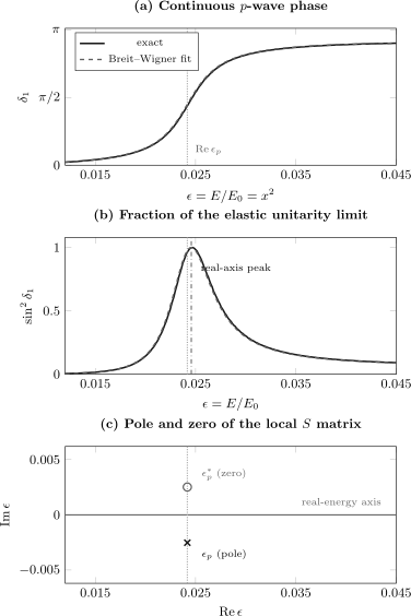
For $g=3.13$, a Breit–Wigner pole factor with a linear background tracks the exact continuous phase over $0.012\le\epsilon\le0.045$. The pole energy $\operatorname{Re}\epsilon_p$ lies below the real-axis point where $\delta_1=\pi/2$ because the background phase is negative. Elastic unitarity pairs the lower-half-plane pole $\epsilon_p$ with an upper-half-plane zero at $\epsilon_p^*$.

Why the Peak Does Not Sit at the Pole Energy

At $\epsilon=\epsilon_{\mathrm{BW}}$, the resonant phase is $\pi/2$, but the total phase is

$$\delta_1 = \frac{\pi}{2} + \delta_{\mathrm{bg}}.$$

For a constant background over the immediate peak region, imposing $\delta_1=\pi/2$ gives

$$\epsilon_{\pi/2} - \epsilon_{\mathrm{BW}} = -\frac{\gamma_{\mathrm{BW}}}{2} \tan\delta_{\mathrm{bg}}.$$

Because $b_0\simeq-0.155$, the right-hand side is positive. The phase peak is shifted upward in energy, exactly as the numerical solution shows.

Three nearby but distinct energies are therefore

$$\begin{aligned} \operatorname{Re}\epsilon_p &= 0.02417497, \\ \epsilon_{\sigma,\max} &= 0.02443760, \\ \epsilon_{\pi/2} &= 0.02457244. \end{aligned}$$

Quoting any one of these without its definition invites a convention error.

Physical Interpretation

Temporary trapping

The well supplies an interior attractive region. For $\ell=1$, the centrifugal contribution

$$\frac{\hbar^2\ell(\ell+1)}{2\mu r^2}$$

separates that region from large radius. Near $g=\pi$, the interior supports a state close to the continuum threshold. Leakage through the barrier gives the state a finite width.

Motion as the depth is tuned

For $g$ below $\pi$, the pole is off the imaginary momentum axis and represents a resonance. As the well is deepened toward the $p$-wave threshold, the pole approaches zero energy and its coupling to the continuum is suppressed. After the state crosses threshold, it becomes a true bound state on the physical sheet.

The near-threshold decay of a short-range $p$ wave carries the Wigner threshold factor $k^{2\ell+1}=k^3$. This explains why a centrifugal-barrier resonance can become narrow as it approaches threshold. A constant-width Breit–Wigner form is only local; it must not be extrapolated all the way to $k=0$.

Phase motion is primary

On the real axis, $|S_1|=1$ throughout. The resonance does not make the elastic $S$ matrix large in magnitude. Instead, it drives $S_1$ rapidly around the unit circle, or equivalently advances $\delta_1$ by nearly $\pi$ across the feature.

The Wigner–Smith delay in this partial wave is

$$\tau_1(E) = 2\hbar \frac{d\delta_1}{dE}.$$

Its large positive value near the resonance expresses temporary trapping. The peak delay of an ideal constant-width pole is $4\hbar/\Gamma$, not $\hbar/\Gamma$; the two times characterize different questions and should not be identified.

Cross-Checks and Error Budget

Exact unitarity

For real energy, verify numerically that

$$|S_1|^2-1$$

is consistent with roundoff. This catches sign errors in $\widehat n_1$, incorrect phase conventions, and inconsistent derivatives.

Threshold law

Away from the tuned resonance region and as $x\to0$,

$$\delta_1=O(x^3),$$

so

$$\sigma_1=O(k^4).$$

A calculation that produces a nonzero constant $p$-wave cross section at threshold has lost the centrifugal suppression.

Pole residual

Substitution of the quoted $x_p$ into the outgoing logarithmic-derivative equation leaves a complex residual below $3\times10^{-15}$ in double precision. This checks the root solver, but not the physical sheet convention; that must be fixed independently by the outgoing boundary condition.

Fit systematics

The numerical integration error is absent because the matching formula is analytic. The relevant uncertainties are instead methodological:

• phase unwrapping and branch consistency;
• fit-window choice;
• background order;
• energy weighting;
• numerical resolution of the complex root;
• the decision to model one isolated pole.

In experimental work, detector response, channel coupling, statistical covariance, and calibration add further layers. The tiny residual here should not be mistaken for a generic experimental precision.

Scope and Limitations

This benchmark assumes one elastic channel and a real central potential. There is no absorption parameter and no branching fraction. In a multichannel problem,

$$S_\ell = \eta_\ell e^{2i\delta_\ell}, \qquad 0\le\eta_\ell\le1,$$

and a resonance width separates into partial widths. See Multichannel Scattering Preview for that extension.

The square well also has a discontinuous boundary and is not a precision model of a particular atom, nucleus, or molecule. Its value is diagnostic: exact matching, exact unitarity, a controllable barrier resonance, and an independently calculable pole are all available in one model.

Common Mistakes

• Treating a width measured in $x=kR$ as an energy width. Because $\epsilon=x^2$, the conversion is nonlinear.
• Calling the $\delta_1=\pi/2$ crossing the pole energy without checking the background phase.
• Fitting only $\sin^2\delta_1$ and losing phase-branch information.
• Omitting a smooth background because the line shape looks nearly symmetric.
• Maximizing $\sin^2\delta_1$ and $\sigma_1$ as if they were the same operation.
• Using $\widehat h_1^{(2)}$ instead of the outgoing $\widehat h_1^{(1)}$ for the chosen time convention.
• Searching for a resonance pole on the real axis, where elastic unitarity keeps $S_1$ finite.
• Interpreting a Gamow state as a normalizable bound-state wavefunction.
• Extrapolating a constant width through the $p$-wave threshold.
• Reporting a fit without the window, weighting, background model, and energy convention.

Cross-Links

• Worked Problems and Model Calculations
• Square-Well Scattering
• Resonances
• Breit–Wigner Form
• Phase Shifts
• Partial-Wave Cross Sections
• Unitarity
• Bound States and Scattering Poles
• Low-Energy S-Wave Scattering
• Phase Shift Extraction

References

• G. Breit and E. Wigner, “Capture of Slow Neutrons,” Physical Review 49, 519–531 (1936), doi:10.1103/PhysRev.49.519.
• E. P. Wigner, “Lower Limit for the Energy Derivative of the Scattering Phase Shift,” Physical Review 98, 145–147 (1955), doi:10.1103/PhysRev.98.145.
• J. R. Taylor, Scattering Theory: The Quantum Theory of Nonrelativistic Collisions, Dover, 2006.
• R. G. Newton, Scattering Theory of Waves and Particles, 2nd ed., Dover, 2002.
• C. J. Joachain, Quantum Collision Theory, 3rd ed., North-Holland, 1983.
• H. M. Nussenzveig, Causality and Dispersion Relations, Academic Press, 1972.
• Particle Data Group, “Resonances,” in Review of Particle Physics, 2025 update, review article.
• L. D. Landau and E. M. Lifshitz, Quantum Mechanics: Non-Relativistic Theory, 3rd ed., Pergamon, 1977.

Exercises

1. Recover the unitary S matrix

Starting from $\tan\delta_1=\mathcal A/\mathcal B$, derive

$$S_1 = \frac{\mathcal B+i\mathcal A} {\mathcal B-i\mathcal A}$$

and prove $|S_1|=1$ for real energy.

Solution

Use

$$e^{2i\delta} = \frac{1+i\tan\delta}{1-i\tan\delta}.$$

Substituting $\tan\delta_1=\mathcal A/\mathcal B$ gives

$$S_1 = \frac{\mathcal B+i\mathcal A} {\mathcal B-i\mathcal A}.$$

At real energy, $\mathcal A$ and $\mathcal B$ are real. The numerator is therefore the complex conjugate of the denominator, so

$$|S_1|^2 = \frac{\mathcal A^2+\mathcal B^2} {\mathcal A^2+\mathcal B^2} = 1.$$

2. Convert the half-maximum width

Use $x_-=0.1494166038$ and $x_+=0.1663625108$ to compute the width in $\epsilon=x^2$. Compare it with $\gamma_p=0.00504455318$.

Solution

Squaring the two momenta gives

$$\begin{aligned} \epsilon_- &= 0.02232532148, \\ \epsilon_+ &= 0.02767648500. \end{aligned}$$

Hence

$$\Delta\epsilon_{1/2} = 0.00535116351.$$

The ratio to the pole width is

$$\frac{\Delta\epsilon_{1/2}}{\gamma_p} = 1.06078.$$

The half-maximum width is about $6.1\%$ larger because the observable contains a background phase and is not an isolated zero-background Lorentzian.

3. Derive the peak shift from a background phase

Assume $\delta_{\mathrm{bg}}$ is constant across the immediate peak. Derive the energy at which the total phase equals $\pi/2$.

Solution

The condition is

$$\delta_{\mathrm{res}} = \frac{\pi}{2} - \delta_{\mathrm{bg}}.$$

Using

$$\tan\delta_{\mathrm{res}} = \frac{\gamma/2} {\epsilon_{\mathrm{BW}}-\epsilon},$$

and $\tan(\pi/2-\delta_{\mathrm{bg}})=\cot\delta_{\mathrm{bg}}$ gives

$$\epsilon_{\pi/2} - \epsilon_{\mathrm{BW}} = -\frac{\gamma}{2} \tan\delta_{\mathrm{bg}}.$$

For a negative background, the phase crossing lies above the Breit–Wigner energy parameter.

4. Convert the momentum pole to energy

Square

$$x_p = 0.1556938588 - 0.0081001159\,i$$

and extract the dimensionless width.

Solution

For $x_p=a-ib$,

$$x_p^2 = (a^2-b^2) - 2iab.$$

Substitution gives

$$x_p^2 = 0.02417496578 - 0.00252227659\,i.$$

Comparing with $\epsilon_p=\epsilon_p^{(R)}-i\gamma_p/2$ yields

$$\begin{aligned} \gamma_p &= 2(0.00252227659) \\ &= 0.00504455318. \end{aligned}$$

5. Diagnose the constant-background bias

The fit with a linear background gives $\gamma=0.00505026710$, while the constant-background fit gives $\gamma=0.00519621390$. Compute both errors relative to the exact pole width.

Solution

For the linear background,

$$\frac{ \gamma_{\mathrm{linear}}-\gamma_p }{ \gamma_p } = 0.113\%.$$

For the constant background,

$$\frac{ \gamma_{\mathrm{constant}}-\gamma_p }{ \gamma_p } = 3.01\%.$$

The more restrictive background model worsens both the residual and the width estimate.

6. Explain the pole–zero pair

Why does the local elastic factor have a pole at $\epsilon_p=\epsilon_R-i\gamma/2$ and a zero at $\epsilon_p^*$?

Solution

The local factor is

$$S_{\mathrm{res}}(\epsilon) = \frac{ \epsilon-\epsilon_R-i\gamma/2 }{ \epsilon-\epsilon_R+i\gamma/2 }.$$

Its denominator vanishes at

$$\epsilon = \epsilon_R-i\gamma/2 = \epsilon_p,$$

while its numerator vanishes at the conjugate point $\epsilon_p^*$. For real $\epsilon$, numerator and denominator are conjugates, which guarantees $|S_{\mathrm{res}}|=1$. The lower-half-plane pole encodes decay for the $e^{-iEt/\hbar}$ convention.