Hard-Sphere Scattering

Hard-sphere scattering is an exact boundary-value problem, not a weak-potential problem. It is therefore a clean test of partial waves, unitarity, threshold expansions, diffraction, and the quantum-to-classical comparison.

Three area scales appear for the same radius $R$:

$$\begin{aligned} \sigma_{\mathrm{quantum}}(kR\ll1) &\longrightarrow 4\pi R^2, \\ \sigma_{\mathrm{classical}} &= \pi R^2, \\ \sigma_{\mathrm{quantum}}(kR\gg1) &\longrightarrow 2\pi R^2. \end{aligned}$$

These are not contradictory answers. They refer to different wave regimes, and the high-energy quantum result still contains a forward diffraction contribution absent from a purely ray-based count.

Partial-Wave Cross Sections owns the general channel sums. This page owns the complete hard-sphere calculation and the comparison among the three limits.

Problem Statement

For relative motion with reduced mass $\mu$, the formal potential is

$$V(r) = \begin{cases} +\infty, & r<R, \\ 0, & r>R. \end{cases}$$

The infinity is shorthand for an excluded region and a Dirichlet boundary condition:

$$u_\ell(R)=0.$$

The physical radial domain is $r\ge R$. For positive energy,

$$E=\frac{\hbar^2k^2}{2\mu},$$

define the only dimensionless control parameter

$$x=kR.$$

The goals are to:

1. derive every exact phase shift $\delta_\ell(x)$;
2. sum the elastic partial cross sections;
3. obtain the low-energy scattering length and effective range;
4. derive the classical differential cross section;
5. explain why the high-energy quantum limit is twice the geometric area.

Because the core is impenetrable, no Born expansion in the potential strength exists. Boundary matching is the natural exact method.

Exact Boundary Phase Shifts

Outside the sphere, the reduced radial equation is free:

$$\left[ - \frac{\hbar^2}{2\mu} \frac{d^2}{dr^2} + \frac{\hbar^2\ell(\ell+1)}{2\mu r^2} \right] u_\ell(r) = E u_\ell(r).$$

Use the real standing-wave convention

$$\begin{aligned} u_\ell(r) ={}& A_\ell \left[ \widehat j_\ell(kr)\cos\delta_\ell \right. \\ &\left. - \widehat n_\ell(kr)\sin\delta_\ell \right], \end{aligned}$$

where

$$\widehat j_\ell(z)=zj_\ell(z), \qquad \widehat n_\ell(z)=zn_\ell(z).$$

At large $r$,

$$u_\ell(r) \sim A_\ell \sin\left( kr-\frac{\ell\pi}{2}+\delta_\ell \right).$$

Applying $u_\ell(R)=0$ gives

$$\widehat j_\ell(x)\cos\delta_\ell - \widehat n_\ell(x)\sin\delta_\ell = 0.$$

Therefore

$$\tan\delta_\ell(x) = \frac{ \widehat j_\ell(x) }{ \widehat n_\ell(x) } = \frac{ j_\ell(x) }{ n_\ell(x) }.$$

This is the exact hard-sphere phase shift for every partial wave.

Branch convention

The tangent fixes $\delta_\ell$ only modulo $\pi$. Choose the low-energy branch satisfying

$$\delta_\ell(x)\to0 \qquad (x\to0).$$

A numerical implementation can evaluate the numerator and denominator with a two-argument arctangent and unwrap the result continuously. For small positive $x$, $j_\ell(x)$ is positive and $n_\ell(x)$ is negative, so a raw $\operatorname{atan2}$ result near $\pi$ must be shifted by $-\pi$ to reach the physical branch near zero.

Exact S-matrix element

With the spherical Hankel functions

$$h_\ell^{(1)}=j_\ell+in_\ell, \qquad h_\ell^{(2)}=j_\ell-in_\ell,$$

the same boundary condition gives

$$S_\ell(x) = e^{2i\delta_\ell} = - \frac{ h_\ell^{(2)}(x) }{ h_\ell^{(1)}(x) }.$$

For real positive $x$,

$$h_\ell^{(2)}(x) = \left[ h_\ell^{(1)}(x) \right]^*,$$

so

$$|S_\ell|=1.$$

The sphere is perfectly elastic. It redirects probability but does not absorb it.

Exact Cross Sections

The elastic scattering amplitude is

$$f(\theta) = \frac{1}{k} \sum_{\ell=0}^{\infty} (2\ell+1) e^{i\delta_\ell} \sin\delta_\ell P_\ell(\cos\theta).$$

The differential cross section is

$$\frac{d\sigma}{d\Omega} = |f(\theta)|^2.$$

After angular integration,

$$\sigma_{\mathrm{el}} = \frac{4\pi}{k^2} \sum_{\ell=0}^{\infty} (2\ell+1) \sin^2\delta_\ell.$$

The exact boundary formula gives

$$\sin^2\delta_\ell = \frac{ j_\ell^2(x) }{ j_\ell^2(x)+n_\ell^2(x) }.$$

Thus

$$\frac{\sigma_{\mathrm{el}}}{\pi R^2} = \frac{4}{x^2} \sum_{\ell=0}^{\infty} (2\ell+1) \frac{ j_\ell^2(x) }{ j_\ell^2(x)+n_\ell^2(x) }.$$

There is no reaction cross section:

$$\sigma_{\mathrm{reac}}=0, \qquad \sigma_{\mathrm{tot}}=\sigma_{\mathrm{el}}.$$

The equality of total and elastic cross sections is a physical statement about this model, not a general identity for scattering with open inelastic channels.

Low-Energy Limit

For $x\ll1$,

$$j_\ell(x) \sim \frac{x^\ell}{(2\ell+1)!!},$$

and

$$n_\ell(x) \sim - \frac{(2\ell-1)!!}{x^{\ell+1}}.$$

Therefore

$$\tan\delta_\ell \sim - \frac{ x^{2\ell+1} }{ (2\ell-1)!!(2\ell+1)!! }.$$

The first channels behave as

$$\begin{aligned} \delta_0&=-x, \\ \delta_1&=-\frac{x^3}{3}+O(x^5), \\ \delta_2&=-\frac{x^5}{45}+O(x^7). \end{aligned}$$

The exact $s$-wave result follows directly from

$$j_0(x)=\frac{\sin x}{x}, \qquad n_0(x)=-\frac{\cos x}{x},$$

which gives

$$\tan\delta_0=-\tan x.$$

On the branch continuous from zero,

$$\delta_0=-x \pmod{\pi}.$$

Scattering length and effective range

The effective-range expansion is

$$k\cot\delta_0 = - \frac{1}{a} + \frac12r_e k^2 +O(k^4).$$

For the hard sphere,

$$\begin{aligned} k\cot\delta_0 &= -k\cot(kR) \\ &= - \frac1R + \frac{R}{3}k^2 +O(k^4). \end{aligned}$$

Hence

$$a=R, \qquad r_e=\frac{2R}{3}.$$

The scattering length is literally the excluded radius in this special model. That identification is not true for a general finite-range potential.

S-wave cross section

The exact $s$-wave contribution is

$$\sigma_0 = \frac{4\pi}{k^2} \sin^2(kR).$$

Equivalently,

$$\frac{\sigma_0}{\pi R^2} = 4 \frac{\sin^2x}{x^2}.$$

As $x\to0$,

$$\sigma_0\longrightarrow4\pi R^2.$$

The next partial wave is suppressed:

$$\sigma_1 \sim \frac{4\pi R^2}{3}x^4.$$

The total low-energy expansion therefore begins

$$\sigma_{\mathrm{el}} = 4\pi R^2 \left[ 1-\frac{x^2}{3}+O(x^4) \right].$$

At leading order, the amplitude is isotropic:

$$f(\theta)\approx-a=-R,$$

so

$$\frac{d\sigma}{d\Omega} \approx R^2.$$

Integrating over $4\pi$ steradians gives $4\pi R^2$.

Classical Hard-Sphere Scattering

Now treat the incident particle as a point ray that reflects specularly from a rigid sphere. Let $b$ be the impact parameter and $\theta$ the deflection angle.

The collision geometry gives

$$b = R\cos\left(\frac{\theta}{2}\right).$$

For an azimuthally symmetric classical scattering map,

$$\frac{d\sigma_{\mathrm{cl}}}{d\Omega} = \frac{b}{\sin\theta} \left| \frac{db}{d\theta} \right|.$$

Because

$$\left| \frac{db}{d\theta} \right| = \frac{R}{2} \sin\left(\frac{\theta}{2}\right),$$

one finds

$$\begin{aligned} \frac{d\sigma_{\mathrm{cl}}}{d\Omega} &= \frac{ R\cos(\theta/2) }{ 2\sin\theta } R\sin(\theta/2) \\ &= \frac{R^2}{4}. \end{aligned}$$

The classical differential cross section is also isotropic, but it is four times smaller than the low-energy quantum result:

$$\left. \frac{d\sigma}{d\Omega} \right|_{\mathrm{quantum},\,x\ll1} = R^2,$$

whereas

$$\left. \frac{d\sigma}{d\Omega} \right|_{\mathrm{classical}} = \frac{R^2}{4}.$$

Integrating the classical result,

$$\sigma_{\mathrm{cl}} = 4\pi\frac{R^2}{4} = \pi R^2.$$

This is the geometric area of impact parameters with $b<R$.

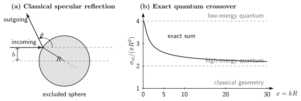
Left: classical geometry gives $b=R\cos(\theta/2)$ and $d\sigma_{\mathrm{cl}}/d\Omega=R^2/4$. Right: the exact quantum partial-wave sum starts at $4\pi R^2$ for $kR\ll1$ and approaches $2\pi R^2$, while the classical geometric cross section is $\pi R^2$.

High-Energy Quantum Limit

When $x=kR\gg1$, partial waves with

$$\ell\lesssim kR$$

probe the sphere. Semiclassically, the angular momentum is related to impact parameter by

$$\ell+\frac12\approx kb.$$

Channels with $\ell\gg kR$ correspond to $b\gg R$ and barely feel the boundary.

For the contributing channels, the exact phase shifts vary rapidly with $\ell$. Averaging the oscillatory factor gives

$$\sin^2\delta_\ell\longrightarrow\frac12$$

in the leading integrated estimate. Let $L\sim kR$. Then

$$\sum_{\ell=0}^{L}(2\ell+1) =(L+1)^2 \sim (kR)^2.$$

The total elastic cross section becomes

$$\begin{aligned} \sigma_{\mathrm{el}} &\sim \frac{4\pi}{k^2} \frac12 (kR)^2 \\ &= 2\pi R^2. \end{aligned}$$

The exact approach includes grazing partial waves and finite-$x$ corrections, so it is slow rather than an abrupt step.

Why the answer is not the classical area

One contribution of order $\pi R^2$ is associated with ordinary reflection from the sphere. A second contribution of the same integrated size comes from forward diffraction generated by the excluded shadow.

The forward peak narrows as $kR$ grows, so it can be missed if one examines only fixed nonzero angles. Nevertheless, its integrated area remains finite and its forward imaginary amplitude is required by the Optical Theorem:

$$\sigma_{\mathrm{tot}} = \frac{4\pi}{k} \operatorname{Im}f(0).$$

Thus the high-energy result

$$\sigma_{\mathrm{tot}}\to2\pi R^2$$

is a wave effect. It does not say that rays with $b>R$ strike the sphere.

Numerical Partial-Wave Audit

The exact sum was evaluated with

$$L_{\max} = \left\lceil x+35 \right\rceil,$$

using 30-digit internal evaluation of the spherical Bessel functions. The large buffer is deliberately conservative; the convergence check below shows that far fewer channels are needed.

$x=kR$	$\sigma_{\mathrm{el}}/(\pi R^2)$
$0.10$	$3.98681618$
$0.30$	$3.89116268$
$1.00$	$3.38243785$
$3.00$	$2.80517768$
$5.00$	$2.60237640$
$10.00$	$2.39722856$
$20.00$	$2.25753111$
$30.00$	$2.19881989$

The values interpolate smoothly between the two quantum limits. At $x=0.10$, the $\ell=0$ contribution is

$$\frac{\sigma_0}{\pi R^2} = 3.98668443,$$

while the $\ell=1$ contribution is only

$$\frac{\sigma_1}{\pi R^2} = 1.31749\times10^{-4}.$$

This directly verifies $s$-wave dominance.

Channel-cutoff convergence at x = 10

$L_{\max}$	$\sigma_{\mathrm{el}}/(\pi R^2)$
$6$	$0.79726341$
$8$	$1.93749006$
$10$	$2.37699286$
$12$	$2.39711918$
$14$	$2.39722847$
$16$	$2.39722856$
$20$	$2.39722856$

Stopping at $\ell=x$ captures most but not all of the answer. The grazing transition extends a few channels beyond $kR$, and a reproducible calculation must demonstrate that this tail is negligible.

The Three Areas Compared

Regime	Differential picture	Total cross section
$kR\ll1$ quantum	coherent isotropic $s$ wave	$4\pi R^2$
classical rays	specular reflection from $b<R$	$\pi R^2$
$kR\gg1$ quantum	specular reflection plus forward diffraction	$2\pi R^2$

The classical result is not obtained by taking the wavelength to zero at every angle and then integrating. The forward diffraction peak becomes distributionally narrow in that limit, so angular integration and the pointwise limit do not commute.

This is the same logic behind many extinction and shadow-diffraction effects: a feature can disappear at every fixed nonzero angle while retaining a finite integrated contribution near the forward direction.

Validity and Scope

The hard-sphere solution is exact for:

• nonrelativistic relative motion;
• a perfectly impenetrable spherical boundary;
• one elastic channel;
• a central interaction with no spin dependence;
• distinguishable particles, or particles whose exchange symmetry is handled separately.

A finite repulsive potential approximates a hard sphere only when penetration is negligible over the energy range of interest. At sufficiently high energy, a finite barrier becomes transparent, whereas the ideal hard sphere remains impenetrable. Its $kR\to\infty$ limit should therefore not be transferred blindly to a finite-height microscopic core.

For identical particles, the amplitude must be symmetrized or antisymmetrized:

$$f_\pm(\theta) = f(\theta)\pm f(\pi-\theta).$$

The allowed partial waves and normalization of the integrated cross section then depend on spin and counting conventions. Those exchange effects are outside this spinless distinguishable-particle calculation.

Common Mistakes

• Treating the formal $+\infty$ potential as an ordinary function rather than a boundary condition.
• Applying the Born approximation to an impenetrable core.
• Using $u_\ell(0)=0$ as the only condition while forgetting $u_\ell(R)=0$ on the exterior domain.
• Writing $\tan\delta_\ell=n_\ell/j_\ell$ instead of $j_\ell/n_\ell$.
• Losing the phase branch when a one-argument arctangent jumps.
• Omitting the $(2\ell+1)$ degeneracy factor.
• Truncating the sum at a fixed $L_{\max}$ as $kR$ increases.
• Calling $\pi R^2$ the universal quantum answer because it is the geometric area.
• Calling $4\pi R^2$ a violation of geometry or probability conservation.
• Dropping the narrow forward diffraction contribution before integrating the high-energy cross section.
• Confusing a perfectly reflecting hard sphere with an absorbing black disk; both show diffraction, but their channel $S$-matrices differ.

Exercises

1. Derive the exact phase shift

Apply the hard boundary condition to the exterior standing-wave solution and derive

$$\tan\delta_\ell = \frac{j_\ell(x)}{n_\ell(x)}.$$

Solution

At $r=R$,

$$0 = \widehat j_\ell(x)\cos\delta_\ell - \widehat n_\ell(x)\sin\delta_\ell.$$

Move the second term to the other side:

$$\widehat n_\ell(x)\sin\delta_\ell = \widehat j_\ell(x)\cos\delta_\ell.$$

Therefore

$$\tan\delta_\ell = \frac{ \widehat j_\ell(x) }{ \widehat n_\ell(x) }.$$

Because both Riccati functions contain the same factor $x$,

$$\tan\delta_\ell = \frac{j_\ell(x)}{n_\ell(x)}.$$

2. Recover the threshold hierarchy

Use the small-$x$ forms of $j_\ell$ and $n_\ell$ to derive the leading power of $\delta_\ell$.

Solution

The ratio is

$$\begin{aligned} \tan\delta_\ell &\sim \frac{ x^\ell/(2\ell+1)!! }{ -(2\ell-1)!!/x^{\ell+1} } \\ &= - \frac{ x^{2\ell+1} }{ (2\ell-1)!!(2\ell+1)!! }. \end{aligned}$$

Since the phase shift is small, $\tan\delta_\ell\sim\delta_\ell$. The $s$, $p$, and $d$ waves therefore begin at orders $x$, $x^3$, and $x^5$.

3. Find the effective range

Starting from $\delta_0=-kR$, derive $a=R$ and $r_e=2R/3$.

Solution

Use

$$\cot z = \frac1z-\frac z3+O(z^3).$$

Then

$$\begin{aligned} k\cot\delta_0 &= -k\cot(kR) \\ &= - \frac1R + \frac{R}{3}k^2 +O(k^4). \end{aligned}$$

Comparing with

$$k\cot\delta_0 = - \frac1a + \frac12r_e k^2 +O(k^4)$$

gives

$$a=R, \qquad r_e=\frac{2R}{3}.$$

4. Derive the classical cross section

Use $b=R\cos(\theta/2)$ to show that the classical differential cross section is isotropic and integrates to $\pi R^2$.

Solution

Differentiate:

$$\frac{db}{d\theta} = - \frac R2 \sin\left(\frac\theta2\right).$$

Then

$$\begin{aligned} \frac{d\sigma_{\mathrm{cl}}}{d\Omega} &= \frac{b}{\sin\theta} \left| \frac{db}{d\theta} \right| \\ &= \frac{ R\cos(\theta/2) }{ 2\sin\theta } R\sin(\theta/2) \\ &= \frac{R^2}{4}. \end{aligned}$$

The integral is

$$\sigma_{\mathrm{cl}} = \int d\Omega\, \frac{R^2}{4} = \pi R^2.$$

5. Estimate the high-energy total

Assume $\sin^2\delta_\ell$ averages to $1/2$ for $0\le\ell\le L$ with $L\approx kR$. Derive the leading total cross section.

Solution

Insert the average into the partial-wave sum:

$$\begin{aligned} \sigma_{\mathrm{el}} &\approx \frac{4\pi}{k^2} \frac12 \sum_{\ell=0}^{L}(2\ell+1) \\ &= \frac{2\pi}{k^2}(L+1)^2. \end{aligned}$$

With $L+1\sim kR$,

$$\sigma_{\mathrm{el}} \longrightarrow 2\pi R^2.$$

The estimate fixes the leading area but not the finite-$kR$ correction from grazing channels.

6. Explain the factor of two

Why does the high-energy quantum cross section not approach the classical geometric area pointwise under angular integration?

Solution

Away from the forward direction, the quantum distribution approaches the ray picture. Near $\theta=0$, however, the excluded shadow produces a diffraction peak. As $kR$ increases, that peak becomes narrower and taller. It can vanish from any fixed nonzero angle while retaining an integrated area of order $\pi R^2$.

The limiting angular distribution is therefore not uniform, and taking the fixed-angle limit before integrating discards the forward contribution. Classical reflection supplies one geometric area and diffraction supplies the second, giving $2\pi R^2$.

Cross-Links

• Radial Schrödinger Equation
• Partial-Wave Expansion
• Phase Shifts
• Partial-Wave Cross Sections
• Scattering Length
• Low-Energy Scattering
• Low-Energy S-Wave Scattering
• Optical Theorem
• Unitarity
• Square-Well Scattering
• Phase Shift Extraction Notebook
• Bessel Functions

References

• J. R. Taylor, Scattering Theory: The Quantum Theory of Nonrelativistic Collisions, Dover, 2006.
• R. G. Newton, Scattering Theory of Waves and Particles, 2nd ed., Dover, 2002.
• C. J. Joachain, Quantum Collision Theory, 3rd ed., North-Holland, 1983.
• L. D. Landau and E. M. Lifshitz, Quantum Mechanics: Non-Relativistic Theory, 3rd ed., Pergamon, 1977.
• R. G. Sachs, Nuclear Theory, Addison-Wesley, 1953.