Lasers

A laser is a driven, dissipative oscillator that converts pump energy into a selected optical field. In the conventional picture, a pumped medium provides gain, feedback returns part of the field to that medium, and saturation establishes a steady state in which gain balances loss. The useful output is the fraction deliberately coupled out of this circulating or traveling field.

The expansion of the name, “light amplification by stimulated emission of radiation,” identifies the microscopic gain process but not the complete device. Stimulated emission can occur in a single-pass amplifier that never oscillates. A passive resonator can store a field but cannot replenish its losses. A working laser combines an energy source, an amplifying response, mode selection, feedback or an equivalent distributed return mechanism, and loss.

This distinction supports a practical definition:

An ordinary optical laser is a self-sustained source whose above-threshold field is selected by the joint dynamics of a pumped gain medium and an optical feedback structure.

The definition is deliberately broader than two mirrors around an inverted atomic transition. Semiconductor gain, distributed-feedback structures, fiber rings, microresonators, and other architectures implement the same oscillator logic differently. Specialized sources such as superradiant or random lasers require refinements, but they do not make every bright source a laser.

Canonical Scope

This page is the conceptual map of laser physics. It owns:

1. the distinction among an optical amplifier, amplified spontaneous emission, a passive cavity, and a laser oscillator;
2. the operating loop from pumping through gain and feedback to saturated output;
3. the qualitative meaning of threshold, coherence, linewidth, pulsed operation, and frequency-comb operation;
4. the limits of describing laser output as a perfectly monochromatic coherent state;
5. the role of lasers as sources, clocks, rulers, force actuators, and Hamiltonian controls in AMO experiments.

The detailed microscopic and measurement theories remain canonical on neighboring pages:

• Stimulated Emission owns occupation-enhanced downward transitions, gain cross sections, inversion, saturation, and amplifier noise.
• Einstein Coefficients owns the $A$ and $B$ coefficients, degeneracy factors, and thermal detailed-balance relations.
• Optical Bloch Equations owns the coherently driven two-level response, relaxation, dephasing, and power broadening.
• Coherent Light owns coherent states, phase references, counting statistics, and the quantum-state caveats for propagating laser fields.
• Input–Output Theory Overview owns the relation between intracavity operators and traveling input and output fields.
• Cavity QED owns coherent emitter–resonator coupling and the distinction between weak and strong coupling.

Laser Principles develops the first quantitative round-trip model. Population Inversion explains how two-, three-, and four-level population cycles produce or fail to produce material gain. Gain and Threshold builds the full modal round-trip loss budget. Optical Cavities develops resonator geometry, free spectral range, linewidth, finesse, quality factor, and stability. Rate-Equation Lasers develops population and photon dynamics. Laser Modes owns longitudinal, Hermite–Gaussian, and Laguerre–Gaussian structure and nonlinear mode competition. Linewidth and Coherence develops phase diffusion, quantum and technical frequency noise, linewidth measurement, and stabilization metrics. Mode Locking develops coherent pulse trains, Frequency Combs develops phase-coherent optical rulers, and Semiconductor Lasers Overview develops diode gain, external cavities, and AMO source design, while Laser Stabilization develops reference discriminators and feedback-loop noise transfer. The present overview supplies the shared vocabulary without duplicating those derivations.

Convention Ledger

Laser formulas are unusually sensitive to whether they describe field amplitudes, powers, angular frequencies, or ordinary frequencies. This page uses:

• $\omega=2\pi\nu$ for angular and ordinary optical frequency;
• $I$ for cycle-averaged intensity or circulating power density;
• $g(\omega,I)$ for a power-gain coefficient in $\mathrm{length}^{-1}$;
• $\alpha_{\mathrm i}$ for distributed internal power loss in $\mathrm{length}^{-1}$;
• $R_j$ and $T_j$ for mirror power reflectivity and transmissivity;
• $L$ for the one-way length of a uniform linear gain region;
• $\mathcal G_{\mathrm{rt}}$ for the round-trip power multiplier;
• $\tau_p$ for photon or energy decay time in the resonator;
• $\kappa$ for an energy-decay rate when that notation is used;
• $g^{(1)}(\tau)$ for normalized first-order temporal coherence;
• $\Delta\nu$ for a spectral full width at half maximum unless stated otherwise.

An amplitude reflectivity is not a power reflectivity, a field-decay rate is not always an energy-decay rate, and a linewidth in rad s$^{-1}$ is not the same numerical quantity as one in Hz. Every detailed calculation must declare these choices.

The Laser Operating Loop

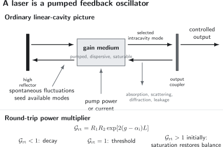
A conventional laser closes an optical feedback loop around a pumped, saturable gain medium. Below threshold a fluctuation decays each round trip; at threshold small-signal gain balances loss; above threshold the field grows until saturation restores round-trip balance. The useful output is also one of the losses that the gain must replace.

The figure should be read dynamically rather than as a list of parts:

1. Pumping drives the medium away from thermal equilibrium.
2. Spontaneous emission and other fluctuations place small fields into many available modes.
3. Stimulated emission amplifies fields where the medium supplies net gain.
4. Feedback and propagation favor modes satisfying the spatial, spectral, polarization, and phase conditions of the resonator.
5. Threshold is reached when the leading mode no longer decays in the small-signal approximation.
6. Saturation and competition stop unlimited growth and redistribute the available gain.
7. Output coupling extracts a controlled traveling field.

The laser therefore selects a collective field–medium solution. Individual stimulated photons do not independently decide the beam direction, linewidth, or phase.

What Makes Laser Light Special?

No single adjective fully characterizes laser light. The useful combination is controllable concentration in selected optical modes.

Spatial concentration

A well-designed resonator can select a nearly diffraction-limited transverse mode with low divergence and high radiance. This makes the field focusable, couplable into a fiber or cavity, and addressable to a localized atom or ion. Directionality is a resonator and mode-selection property, not a consequence of stimulated emission alone.

The quality of a real beam is often summarized by an $M^2$ factor relative to an ideal Gaussian beam. Calling a source “single mode” should specify whether that means one longitudinal mode, one transverse mode, one polarization, or a particular combination.

Spectral concentration

Laser oscillation usually occupies a narrow portion of the gain bandwidth. The optical carrier can therefore be resolved and stabilized far more precisely than a broadband spontaneous source. Yet no physical laser is exactly monochromatic. Finite observation time, phase diffusion, technical frequency noise, cavity drift, and environmental perturbations all broaden or move the spectrum.

The phrase narrow linewidth is incomplete without:

• a lineshape or noise spectrum;
• an observation time or Fourier-frequency band;
• a statement of whether drift is removed;
• a declared full-width or half-width convention.

Temporal coherence

First-order temporal coherence describes the persistence of field correlations:

$$g^{(1)}(\tau) = \frac{ \left\langle E^{(-)}(t) E^{(+)}(t+\tau) \right\rangle }{ \left\langle E^{(-)}(t) E^{(+)}(t) \right\rangle }.$$

For an ideal stationary field with a Lorentzian power spectrum of FWHM $\Delta\nu$,

$$\left| g^{(1)}(\tau) \right| = \exp \left( -\pi\Delta\nu|\tau| \right).$$

This relation gives an $e^{-1}$ coherence time

$$\tau_c = \frac{1}{\pi\Delta\nu},$$

under that particular definition. Other definitions, spectra, and noise processes give different numerical factors or no single coherence time.

Controlled amplitude, phase, polarization, and timing

Lasers can be tuned, modulated, pulsed, locked, frequency shifted, and delivered in engineered spatial and polarization modes. Those controls turn the source into part of an experimental Hamiltonian. They do not imply that every degree of freedom is simultaneously quiet. A source may have excellent short-term phase coherence but poor long-term absolute accuracy, or low frequency noise but excess amplitude noise.

High occupation is not classicality

Many useful laser modes have $\bar n\gg1$, so replacing the field operator by a complex amplitude is accurate for selected observables. Large occupation alone is not a definition of classicality, however. Bright squeezed light can be nonclassical, and a bright laser can carry technical noise well above vacuum.

Stimulated Emission

For one material transition and one selected field mode,

$$|e;n\rangle \longrightarrow |g;n+1\rangle.$$

The creation operator gives

$$\langle n+1| a^\dagger |n\rangle = \sqrt{n+1}.$$

The transition probability therefore contains an occupation-dependent part proportional to $n$ and a vacuum part proportional to one. The former is stimulated emission; the latter is associated with spontaneous emission into that mode.

Stimulated emission adds excitation to an already occupied mode, including its spatial, spectral, and polarization character. This is the microscopic reason an existing field can be amplified coherently. It does not mean that an identifiable photon is copied. Photons in one mode are indistinguishable, and a phase-preserving amplifier must add quantum noise.

Gain requires competition with absorption

The same radiation also drives upward transitions. For lower- and upper-level number densities $\mathcal N_1$ and $\mathcal N_2$, a simple propagation model has small-signal gain

$$g_0(\omega) = \sigma_e(\omega)\mathcal N_2 - \sigma_a(\omega)\mathcal N_1,$$

where $\sigma_e$ and $\sigma_a$ are effective stimulated-emission and absorption cross sections for the declared mode and polarization.

Positive $g_0$ means that stimulated emission exceeds absorption in that model. Equal cross sections give the familiar inversion condition $\mathcal N_2>\mathcal N_1$. Degenerate manifolds, thermalized sublevels, reabsorption, coherences, and broadband media require a more careful condition.

Gain Medium

A gain medium is matter maintained in a nonequilibrium state from which an optical field can extract energy. The pump may be optical, electrical, chemical, collisional, or supplied through another coherent field. The medium may be a dilute gas, ion-doped crystal, semiconductor junction, molecular system, fiber, or nonlinear optical device.

Three properties matter separately:

Property	Question it answers
gain magnitude	Can amplification overcome all losses?
gain spectrum	Which frequencies can grow?
gain dynamics	How quickly do populations and coherences respond?

Pumping and population flow

For an ordinary population-inversion laser, the pump moves population into an upper laser level while relaxation empties the lower laser level. A directly driven closed two-level transition cannot produce steady inversion in the simplest rate model: absorption and stimulated emission equalize the two populations. Practical three- and four-level schemes use additional states and unequal relaxation times.

Population inversion is the standard route to gain, not a universal theorem for every coherently driven multilevel medium. Interference-based gain without inversion exists under specialized conditions. Such exceptions do not remove the need for a nonequilibrium energy source.

Small-signal gain

Ignoring spontaneous source terms and diffraction, one-dimensional power propagation can be written

$$\frac{dI}{dz} = \left[ g(\omega,I) - \alpha_{\mathrm i} \right] I.$$

If the field is weak enough that the populations are unperturbed, $g(\omega,I)\approx g_0(\omega)$. Uniform coefficients then give

$$I(z) = I(0) \exp \left\{ \left[ g_0(\omega)-\alpha_{\mathrm i} \right]z \right\}.$$

This is an amplifier equation, not yet a laser equation. Oscillation requires the amplified field to return with the appropriate phase and sufficient round-trip magnitude.

Saturation

As the field grows, stimulated transitions change the populations and reduce the available inversion. A common phenomenological form for a homogeneously broadened steady-state medium is

$$g(I) = \frac{g_0}{ 1+I/I_{\mathrm{sat}} }.$$

The saturation intensity $I_{\mathrm{sat}}$ depends on transition strength, relaxation, detuning, polarization, and the intensity convention. The formula is useful but not universal: inhomogeneous broadening, standing-wave holes, pulsed extraction, and multilevel kinetics can produce different behavior.

Saturation is what prevents the linear small-signal equation from predicting unbounded exponential growth. It also couples modes through competition for the same pumped population.

Feedback and Mode Selection

In a simple linear laser, two mirrors return the field through the gain medium. In a ring laser the return path is traveling-wave. Distributed Bragg structures, whispering-gallery resonators, external cavities, and fiber loops implement the same idea with different boundary conditions. Optical Cavities derives the resonance, free-spectral-range, linewidth, finesse, quality-factor, and stability relations for these feedback structures.

Magnitude condition

For a uniform linear cavity in which the field traverses a gain length $L$ twice per round trip, the round-trip power multiplier is

$$\mathcal G_{\mathrm{rt}} = R_1R_2 \exp \left[ 2 \left( g-\alpha_{\mathrm i} \right)L \right].$$

A weak field decays when $\mathcal G_{\mathrm{rt}}<1$ and grows when $\mathcal G_{\mathrm{rt}}>1$. This equation assumes power coefficients, uniform traveling-wave gain on each pass, and no additional lumped losses. Any window, aperture, crystal face, polarizer, or imperfect mode match must also be included.

Phase condition

Returning with sufficient magnitude is not enough. A resonant field must also reproduce its phase after one round trip:

$$\Phi_{\mathrm{rt}}(\omega) = 2\pi q, \qquad q\in\mathbb Z.$$

The phase includes propagation through vacuum and dispersive media as well as reflection phases. For an empty nondispersive linear cavity of optical length $L_{\mathrm{opt}}$, adjacent longitudinal resonances are approximately separated by

$$\Delta\nu_{\mathrm{FSR}} \simeq \frac{c}{2L_{\mathrm{opt}}}.$$

The gain profile determines which cavity resonances can be amplified, while loss, spatial overlap, saturation, and competition determine which of those resonances actually oscillate.

Spatial and polarization selection

A resonator also imposes transverse boundary conditions. Diffraction, apertures, mirror curvature, thermal lensing, astigmatism, and the pumped volume select Gaussian-like or more complicated spatial modes. Anisotropic gain, birefringence, intracavity polarizers, and mirror coatings influence polarization.

“The cavity chooses the mode” is therefore shorthand. The oscillating mode is selected by the combined cavity, gain, loss, dispersion, pump geometry, and nonlinear dynamics.

Threshold and Steady Operation

The small-signal threshold of the simple cavity occurs at

$$\mathcal G_{\mathrm{rt}} = 1.$$

Solving for the material power gain gives

$$\begin{aligned} g_{\mathrm{th}} ={}& \alpha_{\mathrm i} \\ &+ \frac{1}{2L} \ln \left( \frac{1}{R_1R_2} \right). \end{aligned}$$

This relation displays the central engineering balance:

• internal absorption and scattering increase threshold;
• a less reflective output coupler extracts more power but also raises threshold;
• a longer gain path lowers the required gain coefficient only if other losses and mode quality do not worsen;
• the relevant gain is modal gain, including overlap between the field and pumped region.

Below, near, and above threshold

Below threshold, spontaneous emission is amplified and filtered, but the mean selected-mode field decays without continuing noise input. The device may be a bright amplified-spontaneous-emission source and still not be an oscillator.

Near threshold, fluctuations are important and a finite noisy device does not exhibit an infinitely sharp textbook kink. Different operational threshold definitions can be extracted from output power, linewidth, statistics, or the leading dynamical eigenvalue.

Above threshold, the leading mode initially grows from fluctuations. Stimulated depletion then reduces its gain until the saturated round-trip multiplier returns to unity. Additional pump power is converted primarily into output and heat rather than unlimited intracavity growth.

Minimal rate-equation map

A generic single-mode rate model can be organized as

$$\begin{aligned} \dot N &= R_p - \frac{N}{\tau_N} - G(N)S, \\ \dot S &= \beta\frac{N}{\tau_N} + \left[ \Gamma G(N) - \frac{1}{\tau_p} \right]S. \end{aligned}$$

Here $N$ is an effective excited population, $S$ is an intracavity photon number, $R_p$ is the pump rate, $\tau_N$ is a population lifetime, $\tau_p$ is a photon lifetime, $\Gamma$ is an overlap or confinement factor, and $\beta$ is the fraction of spontaneous emission entering the selected mode. Definitions differ among atomic, solid-state, and semiconductor laser models, so these equations are a map rather than a plug-in formula.

The stimulated term removes excitation from the medium and adds photons to the field. Threshold appears when the linear coefficient of $S$ changes sign:

$$\Gamma G(N_{\mathrm{th}}) = \frac{1}{\tau_p}.$$

The source term proportional to $\beta$ seeds the mode and rounds the transition. Multimode competition, coherences, carrier transport, and spatial dependence require richer models.

Rate-Equation Lasers derives these equations, their steady branches, finite-$\beta$ crossover, turn-on delay, and relaxation oscillations with one explicit convention set.

Worked Threshold Example

Consider a uniform linear cavity with

$$\begin{gathered} L=0.30\ \mathrm m, \qquad R_1=0.999, \\ R_2=0.950, \qquad \alpha_{\mathrm i}=0.020\ \mathrm{m}^{-1}. \end{gathered}$$

The required material power-gain coefficient is

$$\begin{aligned} g_{\mathrm{th}} &= 0.020 + \frac{1}{0.60} \ln \left[ \frac{1}{ (0.999)(0.950) } \right] \\ &\simeq 0.107\ \mathrm{m}^{-1}. \end{aligned}$$

If the unsaturated gain is $g_0=0.150\ \mathrm{m}^{-1}$, then

$$\begin{aligned} \mathcal G_{\mathrm{rt}} &= (0.999)(0.950) \\ &\quad\times \exp \left[ 2(0.150-0.020)(0.30) \right] \\ &\simeq 1.026. \end{aligned}$$

The weak field grows by about $2.6\%$ in power per round trip. That number is not the steady-state output growth. As intensity builds, gain saturation drives the net round-trip multiplier back toward one.

Coherence and Linewidth

Laser oscillation produces strong phase correlations over useful times, but it does not create an eternal classical sinusoid.

Phase diffusion

Spontaneous emission and other fluctuations perturb the oscillator phase. Because a free-running oscillator has no restoring force for absolute phase, those perturbations accumulate. In an idealized phase-diffusion model,

$$\left| g^{(1)}(\tau) \right| = e^{-D_\phi|\tau|},$$

which corresponds to a Lorentzian spectrum. With the conventions used above, $D_\phi=\pi\Delta\nu$.

The Schawlow–Townes idea relates an irreducible linewidth scale to spontaneous-emission noise, resonator decay, and output power. Exact prefactors depend on linewidth and decay conventions and can be modified by incomplete inversion, amplitude–phase coupling, dispersion, and multimode structure. Technical frequency noise often dominates the fundamental scale. Linewidth and Coherence gives the convention-explicit derivation and connects the optical line to measured phase- and frequency-noise spectra.

Real noise is frequency dependent

Laser noise is best described by spectra:

• frequency or phase noise versus Fourier frequency;
• relative intensity noise;
• pointing and spatial-mode noise;
• polarization noise;
• timing jitter for pulse trains.

A single quoted linewidth may conceal slow drift, discrete modulation peaks, non-Lorentzian wings, or different behavior at short and long averaging times. Precision experiments therefore report the measurement method, bandwidth, observation time, and reference.

Is laser light a coherent state?

A specified output wave packet can often be modeled well by a coherent state $|\alpha\rangle$, especially for normally operating single-mode lasers over a finite interval and within a declared noise band. This model correctly gives a classical mean field, Poisson counting, and vacuum-level quadrature noise.

It is not a universal density operator for “the laser beam.” A free-running laser has an unobserved or diffusing absolute phase, temporal packets can share correlated phase noise, and real sources have excess amplitude noise, side modes, and technical fluctuations. Whether a coherent-state model is adequate depends on the mode definition, reference, observable, and time scale.

The experimentally meaningful question is not “what is the one true state of all laser light?” It is:

Which multimode field model reproduces the measured correlations in the bandwidth and reference frame relevant to this experiment?

Pulsed Lasers

Laser energy need not emerge as a continuous wave.

Gain switching and Q switching

Gain switching drives the gain rapidly through threshold, producing a pulse as the field builds and depletes the inversion. Q switching stores energy in the gain medium while cavity loss is high, then reduces that loss so the stored energy is released in a short, intense pulse. These mechanisms are primarily energy-storage and transient-threshold processes.

Mode locking

A laser supporting many longitudinal modes becomes mode locked only when their relative phases acquire a stable relation. Periodic constructive interference then concentrates the average power into a pulse train. The mode spacing fixes the repetition rate; coherent bandwidth and spectral phase fix the pulse shape and duration.

Mode Locking derives the finite-mode pulse train, active and passive locking mechanisms, the round-trip master-equation picture, Gaussian and $\operatorname{sech}^2$ time–bandwidth conventions, chirp, pulse characterization, and the connection to ultrafast spectroscopy.

Frequency Combs

A phase-coherent pulse train produces an optical grid controlled by two radio-frequency coordinates: tooth spacing from pulse timing and a common offset from carrier-envelope phase slip. When both are measured or stabilized, the grid links microwave references, continuous-wave optical lasers, and atomic transitions.

Frequency Combs derives the tooth equation, $f$-to-$2f$ self-referencing, tooth-index and beat-sign bookkeeping, two-degree-of-freedom stabilization, transfer-oscillator cancellation, optical frequency division, and the role of combs in optical clocks.

Role in AMO Physics

Lasers are simultaneously preparation devices, probes, force sources, local oscillators, and metrology links.

AMO task	Controlled laser quantity	Relevant failure modes
resolve a transition	carrier frequency and linewidth	drift, sidebands, power broadening
drive a quantum rotation	pulse area and optical phase	detuning, amplitude noise, spatial inhomogeneity
cool an atom	detuning, polarization, direction, intensity	frequency noise, imbalance, magnetic-field errors
trap with an AC Stark shift	intensity and spatial mode	scattering, pointing noise, differential shifts
perform Raman control	relative phase and two-photon detuning	path noise, differential Stark shifts
read out a cavity or interferometer	local-oscillator phase and mode match	shot noise, technical noise, loss
compare optical clocks	stabilized frequency and comb coherence	reference noise, cycle slips, dead time
pump a nonlinear source	pulse energy, spectrum, phase matching	multipair noise, thermal drift, modal impurity

The field model depends on the observable

The same physical laser may be represented at different levels:

1. a deterministic classical field for mean coherent dynamics;
2. a classical stochastic field when technical amplitude or phase noise matters;
3. a quantized input field when shot noise, squeezing, counting, or measurement backaction matters;
4. an explicit driven cavity–gain-medium open system when laser generation and linewidth are themselves the subject.

These descriptions are not competitors. They retain different degrees of freedom. A semiclassical drive can accurately model a Rabi experiment while vacuum modes must still be quantized to model spontaneous decay.

Characterize the field at the sample

The quantity specified at a laser head is not necessarily the quantity experienced by an atom. Fibers, modulators, amplifiers, windows, cavities, and free-space propagation can alter frequency, power, polarization, wavefront, phase noise, and timing.

A reproducible AMO report should identify, as relevant:

• vacuum wavelength or optical frequency and its reference;
• linewidth or frequency-noise spectrum with measurement bandwidth;
• power or irradiance at the interaction region;
• beam waist, propagation direction, and spatial-mode quality;
• polarization in the local quantization-axis basis;
• pulse shape, duration, repetition rate, and chirp;
• relative phase between fields in Raman or interferometric protocols;
• calibration method, uncertainty, drift, and feedback bandwidth.

A Laser Analysis Workflow

1. Name the output mode. Specify frequency band, spatial mode, polarization, direction, and continuous-wave or pulsed operation.
2. Identify the pump and level flow. State how energy enters the medium and what produces gain rather than absorption.
3. Write both round-trip conditions. Check magnitude and phase, including every intended and parasitic loss.
4. Separate small-signal and saturated gain. Small-signal gain determines onset; saturated gain determines steady operation.
5. Check competing modes. Include gain bandwidth, transverse overlap, polarization, spatial hole burning, and nonlinear coupling.
6. Choose the noise description. A linewidth, phase-noise spectrum, relative-intensity-noise spectrum, and timing-jitter spectrum answer different questions.
7. Propagate specifications to the experiment. Model every optical component between the source and sample.
8. Validate with observables. Measure threshold behavior, spectrum, spatial mode, power, correlations, or stability rather than inferring them from the device label.

Common Mistakes

Treating stimulated emission as a complete laser theory

Stimulated emission explains microscopic gain. It does not supply pumping, feedback, a phase condition, mode selection, saturation, or output coupling.

Calling amplified spontaneous emission a laser

Amplified spontaneous emission can be bright, directional, and spectrally narrowed by gain. The diagnostic question is whether a self-consistent mode is sustained by feedback or an equivalent oscillator mechanism.

Using amplitude and power coefficients interchangeably

If a field amplitude is multiplied by $r$, its power is multiplied by $R=|r|^2$. Mixing the two changes logarithmic threshold terms by factors of two.

Saying the gain exceeds loss above threshold

Unsaturated gain may exceed loss before the field grows. In a stable single-mode steady state, saturation normally reduces the net modal gain to the loss. Persistent net gain would imply continuing growth.

Equating threshold with a perfectly sharp kink

Spontaneous emission, finite size, noise, multimode behavior, and the chosen observable round the transition. Threshold is a model-dependent operating point as well as a useful asymptotic concept.

Calling every laser exactly monochromatic and coherent

Real fields have finite linewidth, phase noise, amplitude noise, and finite spatial and temporal mode purity. State the observable and bandwidth.

Confusing longitudinal and transverse single-mode operation

A beam may occupy one transverse mode while oscillating at several longitudinal frequencies, or one longitudinal resonance while carrying an imperfect spatial mode.

Quoting a cavity linewidth without a convention

State whether the width refers to field or power response, HWHM or FWHM, angular frequency or ordinary frequency, and loaded or intrinsic loss.

Cross-Links

• AMO Bibliography and Reading Guide compares laser textbooks, classic theory, spectroscopy sources, and convention cautions.
• Laser Nomenclature is the convention ledger for gain, threshold, finesse, $Q$, mode volume, linewidth, coherence length, Rabi frequency, detuning, and saturation intensity.
• Atoms, Molecules, and Light places lasers within the full AMO preparation–dynamics–measurement loop.
• Light–Matter Interaction develops the microscopic coupling and few-level response.
• Quantum Optics develops field states, transformations, correlations, and detection.
• Line Shapes and Broadening separates natural, Doppler, collisional, power, instrumental, and source contributions.
• Precision Spectroscopy treats calibration, uncertainty, frequency references, and measurement design.
• Lasers and Quantum Technology gives the experimental and historical perspective.

Exercises

1. Classify four optical systems

Classify each system as a passive resonator, optical amplifier, amplified spontaneous-emission source, or laser oscillator.

1. A lossy Fabry–Pérot cavity is illuminated by an external narrowband field.
2. A pumped rare-earth fiber amplifies an injected signal and has angled, antireflection-coated ends.
3. The same pumped fiber emits broadband light from spontaneous photons that are amplified during one pass.
4. The fiber is placed in a ring with a wavelength-selective element and an output coupler; a field persists without an injected signal.

Solution

1. The Fabry–Pérot is a passive resonator. It stores and filters the injected field but supplies no gain.
2. The seeded, reflection-suppressed fiber is an optical amplifier.
3. The unseeded one-pass output is amplified spontaneous emission.
4. The closed-loop device is a laser oscillator because a selected mode is sustained by gain and feedback without an external seed.

Brightness or directionality alone did not decide the classification.

2. Find a round-trip threshold

A linear cavity has $L=0.20\ \mathrm m$, $R_1=0.995$, $R_2=0.90$, and $\alpha_{\mathrm i}=0.030\ \mathrm{m}^{-1}$. Find the threshold material power-gain coefficient.

Solution

Use

$$g_{\mathrm{th}} = \alpha_{\mathrm i} + \frac{1}{2L} \ln \left( \frac{1}{R_1R_2} \right).$$

The reflectivity product is

$$R_1R_2 = (0.995)(0.90) = 0.8955.$$

Therefore

$$\begin{aligned} g_{\mathrm{th}} &= 0.030 + \frac{1}{0.40} \ln \left( \frac{1}{0.8955} \right) \\ &\simeq 0.306\ \mathrm{m}^{-1}. \end{aligned}$$

The result uses power coefficients. Using amplitude reflectivities in the same formula would be inconsistent.

3. Audit an output-coupler change

In the model above, the output-coupler reflectivity is reduced while all other quantities are held fixed. Explain why the threshold rises, why the extractable fraction per encounter rises, and why choosing the smallest possible reflectivity does not generally maximize useful output.

Solution

Reducing $R_2$ increases the logarithmic mirror-loss term,

$$\frac{1}{2L} \ln \left( \frac{1}{R_1R_2} \right),$$

so more material gain is required at threshold. If absorption is negligible, the transmitted fraction $T_2\approx1-R_2$ increases, so a larger fraction of the intracavity power is extracted on each encounter.

These trends compete. Excessive output coupling can raise the required gain beyond what the pump supplies and can greatly reduce circulating power. Excessively weak coupling traps power while internal loss consumes it. The optimum depends on available saturated gain, internal loss, mode overlap, and the desired output rather than on transmissivity alone.

4. Infer a coherence time

A stationary laser has a Lorentzian power spectrum with FWHM $\Delta\nu=100\ \mathrm{kHz}$. Under the convention $|g^{(1)}(\tau)|=\exp(-\pi\Delta\nu|\tau|)$, find the $e^{-1}$ coherence time and the corresponding vacuum propagation length $c\tau_c$.

Solution

The coherence time is

$$\tau_c = \frac{1}{ \pi(100\times10^3\ \mathrm{s}^{-1}) } \simeq 3.18\ \mu\mathrm s.$$

Using $c\simeq2.998\times10^8\ \mathrm{m\,s}^{-1}$,

$$c\tau_c \simeq 9.54\times10^2\ \mathrm m.$$

This is about $954\ \mathrm m$. It is a correlation length for the declared stationary Lorentzian model, not necessarily the distance over which an unstabilized experiment retains a known absolute phase.

5. Diagnose a coherent-state claim

An experimenter says, “The beam is from a single-frequency laser, so every one-microsecond temporal packet is an independent pure coherent state with the same known phase.” Identify at least three unsupported parts of the claim.

Solution

“Single frequency” normally means that one longitudinal component dominates within a stated resolution. It does not prove zero linewidth or a perfectly pure spatial, polarization, and temporal mode.

A free-running laser need not have a known absolute phase. A phase reference or a preparation record is required to operationally define that phase.

Successive packets are not necessarily independent. They can share phase diffusion, amplitude noise, pump noise, and servo correlations.

Finally, a coherent-state model requires suitable counting and quadrature statistics in the relevant bandwidth. The device label alone does not establish a pure coherent density operator.

6. Distinguish pulsed-laser mechanisms

For gain switching, Q switching, and mode locking, identify the principal quantity being controlled and one diagnostic that distinguishes the regime.

Solution

Gain switching drives gain through threshold and observes the transient field buildup and inversion depletion. The pulse timing follows the pump drive; a time-resolved output versus pump waveform tests the mechanism.

Q switching stores inversion while cavity loss is high and releases it after the loss is reduced. Its pulses are typically separated by an energy-storage timescale rather than one cavity round trip; simultaneous measurement of intracavity loss, inversion proxy, and output pulse distinguishes it.

Mode locking establishes a stable relative phase among many longitudinal modes. A radio-frequency line at the pulse repetition rate together with a broad coherent optical spectrum and phase-sensitive pulse characterization tests this regime. A pulse train alone is insufficient because Q-switched mode locking can place short pulses inside a slower envelope.

7. Choose a laser model for three observables

An atom is driven by a bright laser while fluorescence photons are counted. Choose the minimum useful field description for:

1. the mean Rabi oscillation when source noise is negligible;
2. loss of contrast caused by measured laser-frequency noise;
3. photon-counting shot noise and spontaneous emission into unoccupied modes.

Solution

1. A deterministic classical drive with measured amplitude, phase, and detuning is sufficient for the ideal mean Rabi oscillation.
2. A classical stochastic drive with the measured frequency- or phase-noise process is the minimum model for source-induced contrast loss.
3. The detected output and vacuum reservoir require a quantized-field or equivalent quantum-trajectory description. Treating the strong incident laser semiclassically can still be consistent if its depletion and quantum fluctuations are negligible for the observable.

The correct model is selected by the measurement, not by a rule that the entire electromagnetic field must be represented at one level.

References

1. A. Einstein, “Zur Quantentheorie der Strahlung,” Physikalische Zeitschrift 18, 121–128 (1917). The source of the absorption, spontaneous-emission, and stimulated-emission coefficient framework.
2. A. L. Schawlow and C. H. Townes, “Infrared and Optical Masers,” Physical Review 112, 1940–1949 (1958).
3. T. H. Maiman, “Stimulated Optical Radiation in Ruby,” Nature 187, 493–494 (1960).
4. A. E. Siegman, Lasers, University Science Books (1986).
5. P. W. Milonni and J. H. Eberly, Laser Physics, Wiley (2010).
6. M. Sargent III, M. O. Scully, and W. E. Lamb Jr., Laser Physics, Addison–Wesley (1974).
7. H. Haken, Laser Theory, Springer (1984), doi:10.1007/978-3-642-45551-7.
8. L. Mandel and E. Wolf, Optical Coherence and Quantum Optics, Cambridge University Press (1995), doi:10.1017/CBO9781139644105.
9. R. J. Glauber, “The Quantum Theory of Optical Coherence,” Physical Review 130, 2529–2539 (1963).
10. K. Mølmer, “Optical Coherence: A Convenient Fiction,” Physical Review A 55, 3195–3203 (1997).
11. H. M. Wiseman, “Defining the (Atom) Laser,” Physical Review A 56, 2068–2084 (1997).
12. H. A. Haus, “Mode-Locking of Lasers,” IEEE Journal of Selected Topics in Quantum Electronics 6, 1173–1185 (2000).
13. Th. Udem, R. Holzwarth, and T. W. Hänsch, “Optical Frequency Metrology,” Nature 416, 233–237 (2002).
14. S. T. Cundiff and J. Ye, “Colloquium: Femtosecond Optical Frequency Combs,” Reviews of Modern Physics 75, 325–342 (2003).
15. S. T. Diddams, “The Evolving Optical Frequency Comb,” Journal of the Optical Society of America B 27, B51–B62 (2010).