Linewidth and Coherence

A laser can oscillate in one spatial and longitudinal mode without being perfectly monochromatic. The selected mode fixes a carrier-frequency neighborhood and field pattern; fluctuations of its phase make the emitted line finite. A laser linewidth is therefore not merely a property of a passive cavity resonance. It is an operational summary of temporal coherence, stochastic dynamics, observation time, and measurement method.

The shortest reliable statement is

$$\text{phase fluctuations} \longleftrightarrow \text{decay of }g^{(1)}(\tau) \longleftrightarrow \text{finite optical spectrum}.$$

For ideal white frequency noise, this chain gives an exponential coherence envelope and a Lorentzian line. Real lasers also have drift, flicker noise, mechanical resonances, modulation sidebands, mode hops, and servo features. Then one full width at half maximum cannot encode the complete behavior.

Canonical Scope

This page owns:

1. first-order temporal coherence and its relation to a cw laser spectrum;
2. coherence-time, coherence-length, HWHM, FWHM, hertz, and angular-frequency conventions;
3. Brownian phase diffusion and the resulting Lorentzian line;
4. the relation among phase-noise, frequency-noise, and optical spectra;
5. the Schawlow–Townes idea and a convention-explicit quantum-limited scale;
6. incomplete-inversion, amplitude–phase, and mode-nonorthogonality corrections;
7. technical frequency noise, finite observation time, and non-Lorentzian lines;
8. heterodyne, delayed self-heterodyne, discriminator, and spectrum measurements;
9. the distinction among free-running linewidth, locked linewidth, and long-term frequency stability.

Correlation Functions owns the general quantum-optical hierarchy $G^{(n)}$ and the Wiener–Khinchin theorem. Coherent Light owns coherent states and explains why first-order coherence, Poisson counting, and coherent-state purity are different claims. Optical Cavities owns passive resonator linewidth, photon lifetime, finesse, and $Q$. Line Shapes and Broadening owns atomic and molecular transition widths. The present page applies those ideas specifically to the fluctuating output of a laser oscillator.

Convention Ledger

Factors of two and $2\pi$ cause more linewidth disagreements than new physics. Unless stated otherwise:

• the positive-frequency field is written $\mathcal E^{(+)}(t)=A(t)e^{-i[2\pi\nu_0t+\phi(t)]}$;
• $\nu$ and Fourier offset $f$ are ordinary frequencies in hertz;
• $\omega=2\pi\nu$ is an angular frequency in radians per second;
• $\Delta\nu$ means an optical power-spectrum FWHM in hertz;
• $\kappa$ is the intracavity photon-number decay rate, defined by $\dot n=-\kappa n$ when gain is absent;
• $S_\nu^{(2)}(f)$ is a two-sided classical frequency-noise PSD;
• $S_\nu^{(1)}(f)=2S_\nu^{(2)}(f)$ for $f>0$ is its one-sided version;
• PSD formulas assume stationary noise unless a finite record or explicit low-frequency cutoff is declared.

The instantaneous frequency fluctuation associated with the phase convention above is

$$\delta\nu(t) = \frac{1}{2\pi} \frac{d\phi}{dt}.$$

Changing the sign in the field convention changes the sign of $\delta\nu$, but not any autocorrelation or PSD used below.

Temporal Coherence

First-order correlation

For one selected polarization and detected spatial mode, define

$$G^{(1)}(\tau) = \left\langle \mathcal E^{(-)}(t) \mathcal E^{(+)}(t+\tau) \right\rangle.$$

For a stationary beam, this depends only on the delay $\tau$. Its normalized form is

$$g^{(1)}(\tau) = \frac{ G^{(1)}(\tau) }{ G^{(1)}(0) }.$$

The normalization gives $g^{(1)}(0)=1$ for nonzero mean intensity and $|g^{(1)}(\tau)|\le 1$. In a balanced delayed interferometer, the fringe visibility is $|g^{(1)}(\tau)|$ when polarization, spatial mode, and intensities are matched. Coherence is therefore a relation between two field samples, not a statement that an absolute optical phase is known.

If amplitude noise is negligible on the timescale of interest,

$$\mathcal E^{(+)}(t) \simeq \mathcal E_0 e^{-i[2\pi\nu_0t+\phi(t)]},$$

and

$$g^{(1)}(\tau) = e^{-i2\pi\nu_0\tau} \left\langle e^{-i[\phi(t+\tau)-\phi(t)]} \right\rangle.$$

Only phase increments appear. The absolute phase may diffuse without bound while the increment statistics remain stationary.

Optical spectrum

Use the ordinary-frequency Wiener–Khinchin pair

$$\begin{aligned} S_E(\nu) &= \int_{-\infty}^{\infty} d\tau\, e^{i2\pi\nu\tau} G^{(1)}(\tau), \\ G^{(1)}(\tau) &= \int_{-\infty}^{\infty} d\nu\, e^{-i2\pi\nu\tau} S_E(\nu). \end{aligned}$$

An overall normalization depends on whether $S_E$ is a power, photon-flux, or field spectrum. The line shape and widths do not. For an isolated stationary line, the normalized spectrum

$$\mathcal L(\nu) = \frac{S_E(\nu)} {\int S_E(\nu')\,d\nu'}$$

has units of inverse hertz and integrates to one.

Lorentzian Fourier pair

A Lorentzian with FWHM $\Delta\nu$ is

$$\mathcal L_{\mathrm L}(\nu) = \frac{1}{\pi} \frac{\Delta\nu/2}{ (\nu-\nu_0)^2+(\Delta\nu/2)^2 }.$$

Its normalized field correlation is

$$g_{\mathrm L}^{(1)}(\tau) = e^{-i2\pi\nu_0\tau} e^{-\pi\Delta\nu|\tau|}.$$

Thus the $1/e$ decay time of the field-correlation amplitude is

$$\tau_{1/e} = \frac{1}{\pi\Delta\nu}.$$

The integral convention used on the general correlation page,

$$\tau_c^{(2)} = \int_{-\infty}^{\infty} d\tau\, |g^{(1)}(\tau)|^2,$$

happens to give the same numerical value for a Lorentzian:

$$\tau_c^{(2)} = \frac{1}{\pi\Delta\nu}.$$

That equality is special to the exponential envelope and these integration limits. A one-sided integral, an intensity-correlation width, or a different threshold gives another number.

Gaussian Fourier pair

A normalized Gaussian line with rms width $\sigma_\nu$ is

$$\mathcal L_{\mathrm G}(\nu) = \frac{1}{ \sqrt{2\pi}\sigma_\nu } \exp \left[ -\frac{(\nu-\nu_0)^2}{2\sigma_\nu^2} \right].$$

Then

$$g_{\mathrm G}^{(1)}(\tau) = e^{-i2\pi\nu_0\tau} e^{-2\pi^2\sigma_\nu^2\tau^2},$$

and

$$\Delta\nu_{\mathrm G} = 2\sqrt{2\ln2}\,\sigma_\nu.$$

Slow Gaussian-distributed frequency excursions often create a Gaussian core, while white frequency noise creates Lorentzian wings or a Lorentzian core. Their convolution is Voigt only when the corresponding broadening processes are independent and have the required stationary distributions.

Coherence length

A coherence time becomes a distance only after the propagation geometry is specified. For group velocity $v_g$,

$$\ell_c = v_g\tau_c.$$

In a Michelson interferometer, a mirror displacement $x$ changes the optical path by approximately $2x$, so the mechanical displacement associated with a delay $\tau$ is $x=v_g\tau/2$. Quoting $c/\Delta\nu$ as “the coherence length” without a time definition and path convention can therefore differ from another correct convention by factors of $\pi$ or two.

Three linewidths that must not be conflated

Object	What has a width?	Primary mechanism
passive cavity	driven cavity power response	photon escape and internal loss
material transition	absorption or emission response	radiative, collisional, Doppler, power, and other broadening
laser output	oscillator field spectrum	phase noise plus technical fluctuations

A laser output can be far narrower than both its gain bandwidth and its passive-cavity resonance. Gain replenishes the decaying field amplitude, but it does not restore a unique absolute phase after random phase perturbations.

Phase Diffusion

Why phase is the soft coordinate

Above threshold, gain saturation supplies a restoring tendency for amplitude: if the field grows, it depletes inversion and reduces net gain. A free-running autonomous laser has continuous phase symmetry. Rotating the steady complex amplitude by a constant phase produces an equally valid solution, so there is no analogous restoring force for absolute phase.

A small random quadrature kick has a radial part and a tangential part in complex-amplitude space. The radial part is damped; the tangential part shifts phase. Repeated tangential kicks accumulate into diffusion.

Wiener model

Write the phase stochastic differential equation as

$$d\phi(t) = \sqrt{2D_\phi}\,dW_t,$$

where $dW_t$ is a Wiener increment with

$$\langle dW_t\rangle=0, \qquad \langle dW_t^2\rangle=dt.$$

The phase increment is Gaussian with

$$\left\langle [\phi(t+\tau)-\phi(t)]^2 \right\rangle = 2D_\phi|\tau|.$$

For any zero-mean Gaussian variable $X$,

$$\langle e^{-iX}\rangle = e^{-\langle X^2\rangle/2}.$$

Therefore

$$g^{(1)}(\tau) = e^{-i2\pi\nu_0\tau} e^{-D_\phi|\tau|}.$$

Comparison with the Lorentzian Fourier pair gives

$$D_\phi = \pi\Delta\nu, \qquad \Delta\nu = \frac{D_\phi}{\pi}.$$

Some authors define their diffusion constant by $\langle(\Delta\phi)^2\rangle=D|\tau|$ rather than $2D|\tau|$. The physics is unchanged; the symbol differs by two.

White frequency noise

Define the two-sided frequency-noise PSD by

$$S_\nu^{(2)}(f) = \int_{-\infty}^{\infty} d\tau\, e^{-i2\pi f\tau} \langle \delta\nu(t+\tau)\delta\nu(t) \rangle.$$

Since $\delta\nu=\dot\phi/(2\pi)$,

$$S_\nu^{(2)}(f) = f^2S_\phi^{(2)}(f),$$

away from singular contributions at $f=0$. Equivalently,

$$S_\phi^{(2)}(f) = \frac{S_\nu^{(2)}(f)}{f^2}.$$

Suppose the two-sided frequency-noise PSD is white:

$$S_\nu^{(2)}(f)=h_0.$$

Then its time correlation is $h_0\delta(\tau)$, and integration over a delay gives

$$\left\langle [\phi(t+\tau)-\phi(t)]^2 \right\rangle = 4\pi^2h_0|\tau|.$$

Hence

$$D_\phi = 2\pi^2h_0, \qquad \Delta\nu = 2\pi h_0.$$

For the one-sided white plateau $H_0=2h_0$, the same result is

$$\Delta\nu = \pi H_0.$$

This useful formula is valid only for the declared one-sided PSD in $\mathrm{Hz^2/Hz}$. Applying it to an angular-frequency PSD or a two-sided PSD without conversion gives a wrong factor.

Arbitrary Gaussian frequency noise

For stationary, zero-mean Gaussian frequency noise,

$$\Delta\phi(\tau) = 2\pi \int_t^{t+\tau} \delta\nu(t')\,dt'.$$

Using a one-sided PSD gives

$$\frac12 \left\langle [\Delta\phi(\tau)]^2 \right\rangle = 2 \int_0^\infty df\, S_\nu^{(1)}(f) \frac{ \sin^2(\pi f\tau) }{ f^2 }.$$

Therefore

$$\begin{aligned} g^{(1)}(\tau) ={}& e^{-i2\pi\nu_0\tau} \\ &\times \exp \left[ -2 \int_0^\infty df\, S_\nu^{(1)}(f) \frac{\sin^2(\pi f\tau)}{f^2} \right]. \end{aligned}$$

The optical line follows by Fourier transformation. This relation is more fundamental than assigning each PSD a single “integrated linewidth.” It also shows why low-frequency noise is dangerous: the phase response contains $1/f^2$.

The β-separation estimate

For practical one-sided frequency-noise data, the β-separation line is

$$S_{\nu,\beta}(f) = \frac{8\ln2}{\pi^2}\,f.$$

Noise above this line has a high modulation index and contributes strongly to an approximate FWHM. With record duration $T_0$, define

$$\begin{aligned} A(T_0) = \int_{1/T_0}^{\infty} df\, S_\nu^{(1)}(f) \,\Theta \left[ S_\nu^{(1)}(f) -S_{\nu,\beta}(f) \right]. \end{aligned}$$

The estimate is

$$\Delta\nu_\beta \simeq \sqrt{8\ln2\,A}.$$

This is a useful diagnostic, not an exact replacement for Fourier transforming $g^{(1)}$. Its explicit lower limit exposes the observation-time dependence caused by flicker or random-walk frequency noise. Noise below the β line can still make spectral wings, sidebands, and phase errors important to an application.

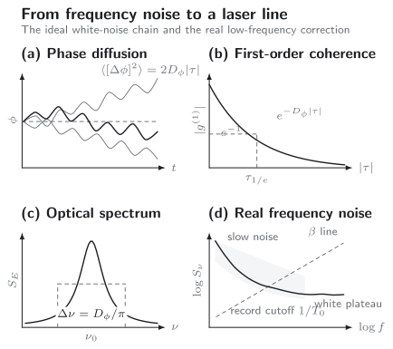
White frequency noise makes the phase execute a random walk. Gaussian phase increments then give an exponential $|g^{(1)}(\tau)|$ and a Lorentzian optical line. Real frequency-noise spectra often rise at low Fourier frequency; the β-separation line is an observation-time-dependent estimate of which components broaden the central line strongly.

Modulation is not diffusion

A deterministic sinusoidal phase

$$\phi(t) = \beta\sin(2\pi f_mt)$$

produces discrete sidebands with Bessel-function weights. It does not by itself produce irreversible phase diffusion. Random modulation, unresolved sidebands, or a finite instrument resolution may make the measured trace look broadened, so line broadening must be distinguished from coherent modulation.

The Schawlow–Townes Idea

Random phasor additions

Stimulated emission adds field in phase with the occupied mode, whereas spontaneous emission into that mode carries an unpredictable quadrature. For a large coherent amplitude of radius $\sqrt{\bar n}$, a transverse fluctuation of fixed scale produces a phase kick proportional to $1/\sqrt{\bar n}$. The phase variance per kick is therefore proportional to $1/\bar n$.

This gives the robust scaling

$$\text{quantum-limited linewidth} \propto \frac{ \text{noise injection rate} }{ \text{intracavity photon number} }.$$

Since output power is proportional to photon number at fixed output coupling, the linewidth narrows approximately as $1/P_{\mathrm{out}}$. The original Schawlow–Townes argument captured this central idea. Modern quantum laser theories are needed to specify which gain and loss processes contribute and to settle convention-dependent factors.

One explicit ideal convention

Consider an ideal single-mode, far-above-threshold, Markovian laser with:

• an adiabatically eliminated gain medium;
• no amplitude–phase coupling;
• an orthogonal cavity mode;
• complete inversion in the effective transition;
• mean intracavity photon number $\bar n\gg1$;
• photon-number loss rate $\kappa$.

In a widely used conventional linear-gain model, the angular-frequency power-spectrum FWHM is

$$\Delta\omega_{\mathrm{SQL}} = \frac{\kappa}{2\bar n}.$$

Because $\Delta\omega=2\pi\Delta\nu$, this page’s ordinary-frequency FWHM is

$$\Delta\nu_{\mathrm{SQL}} = \frac{\kappa}{4\pi\bar n}.$$

Equivalently, the phase-diffusion coefficient is

$$D_\phi = \frac{\kappa}{4\bar n}.$$

The label “standard quantum limit” here names this conventional laser model, not a theorem that no engineered gain process can do better. Quantum gain models with different noise properties require their own derivation.

Express the scale through output power

Let $\kappa_{\mathrm{out}}$ be the photon escape rate through the monitored output port. Then

$$P_{\mathrm{out}} = \hbar\omega_0 \kappa_{\mathrm{out}} \bar n,$$

so

$$\Delta\nu_{\mathrm{SQL}} = \frac{ \hbar\omega_0 \kappa\kappa_{\mathrm{out}} }{ 4\pi P_{\mathrm{out}} }.$$

If output coupling dominates all loss, $\kappa_{\mathrm{out}}\simeq\kappa$. Since the passive cavity FWHM is

$$\Delta\nu_c = \frac{\kappa}{2\pi},$$

the result becomes

$$\Delta\nu_{\mathrm{SQL}} \simeq \frac{ \hbar\omega_0\kappa^2 }{ 4\pi P_{\mathrm{out}} } = \frac{ \pi h\nu_0(\Delta\nu_c)^2 }{ P_{\mathrm{out}} }.$$

Every equality in this chain uses a declared definition. Formulas in the literature can differ because the symbol called “cavity linewidth” may be a field HWHM, power HWHM, power FWHM, or angular-frequency width, and because some derivations use total dissipated power rather than one output port.

Correction map

Real devices can depart from the ideal scale in several conceptually different ways.

Factor or effect	Physical origin	Typical role
$n_{\mathrm{sp}}$	incomplete inversion and excess spontaneous emission	multiplies the ideal diffusion scale in common laser models
$1+\alpha_H^2$	carrier-induced gain fluctuations coupled to refractive-index fluctuations	Henry broadening in semiconductor lasers
$K$	nonorthogonal left and right cavity modes	Petermann excess-noise factor
dispersive pulling	gain or intracavity dispersion changes phase response and group delay	can alter the conversion from noise to frequency
multiple modes	shared gain, mode beating, hopping, and non-normal coupling	can invalidate a one-phase description
technical noise	pumps, mechanics, electronics, temperature, feedback	usually adds a frequency-dependent PSD rather than one constant factor

Under a restricted model, one often encounters the schematic estimate

$$\Delta\nu \simeq \Delta\nu_{\mathrm{SQL}}\, n_{\mathrm{sp}} (1+\alpha_H^2) K.$$

This is a correction map, not a universal product law. The factors can be frequency dependent, correlated, or already included in a more microscopic noise model.

Incomplete inversion

In a simple gain medium with upper- and lower-state populations $N_2$ and $N_1$, a conventionally normalized spontaneous-emission factor has the form

$$n_{\mathrm{sp}} \sim \frac{N_2}{N_2-N_1},$$

when emission and absorption cross sections are treated symmetrically. Complete inversion gives $n_{\mathrm{sp}}\to1$. Near transparency, $N_2-N_1$ becomes small and this simplified factor grows. Actual multilevel and semiconductor expressions must use the relevant gain and occupation model.

Amplitude–phase coupling

In a semiconductor, a carrier fluctuation changes both gain and refractive index. The corresponding phase and amplitude quadratures are coupled. Henry’s linewidth-enhancement parameter $\alpha_H$ measures that coupling in a declared susceptibility or gain convention. In the standard approximation it broadens the intrinsic line by

$$1+\alpha_H^2.$$

The same coupling also produces chirp under current modulation. Semiconductor Lasers Overview defines $\alpha_H$ in an intensity-gain convention and develops its device context. The important lesson here is that amplitude restoration does not prevent amplitude noise from being converted into phase noise.

Mode nonorthogonality

Open, gain-guided, lossy, or otherwise non-Hermitian resonators can have nonorthogonal eigenmodes. For one isolated resonance, the Petermann factor $K\ge1$ quantifies enhanced spontaneous-emission noise associated with the left–right mode overlap. It is not simply a statement that two transverse intensity patterns overlap. Near exceptional points or strongly overlapping resonances, a scalar isolated-mode factor may itself become inadequate.

Where the ideal estimate fails

The far-above-threshold phase-diffusion picture can fail:

• near threshold, where amplitude and phase fluctuations are strongly coupled and the line may be non-Lorentzian;
• in few-emitter or strong-coupling lasers, where adiabatic elimination and Gaussian noise fail;
• in bad-cavity or superradiant lasers, where the active medium stores much of the phase;
• in multimode or mode-hopping operation;
• under delayed optical feedback or injection locking;
• when technical noise exceeds the quantum scale.

A smaller fitted line than a naïve Schawlow–Townes estimate is not by itself a violation of quantum mechanics. First verify that the same definitions, ports, loss rates, operating regime, and gain model were used.

Technical Frequency Noise

Optical-path fluctuations

For a simple cavity resonance,

$$\nu_q \simeq \frac{q c}{2nL},$$

so small optical-path changes give

$$\frac{\delta\nu_q}{\nu_q} \simeq - \left( \frac{\delta L}{L} + \frac{\delta n}{n} \right).$$

Mirror displacement, acoustic vibration, thermal expansion, thermorefractive noise, air-pressure changes, coating fluctuations, and pump-induced thermal lensing can therefore become laser frequency noise. A fractional optical path change of $10^{-15}$ shifts a $300\ \mathrm{THz}$ carrier by about $0.3\ \mathrm{Hz}$.

The cold-cavity relation is only a starting point. Gain dispersion and frequency pulling determine how strongly the lasing frequency follows the cavity and material resonances.

Pump and gain fluctuations

Pump noise changes inversion, gain saturation, temperature, and refractive index. It can produce:

• direct amplitude noise;
• amplitude-to-phase conversion;
• carrier-density chirp in semiconductors;
• thermal frequency drift;
• relaxation-oscillation peaks;
• changes of spatial mode or polarization.

Relative intensity noise is commonly defined as

$$S_{\mathrm{RIN}}(f) = \frac{ S_P^{(1)}(f) }{ \bar P^2 },$$

with units $\mathrm{Hz^{-1}}$. Pure amplitude noise does not automatically broaden the optical carrier, but nonlinear index changes, detector conversion, saturation, and semiconductor $\alpha_H$ coupling can turn it into phase noise.

Feedback and back reflections

Unintended optical feedback returns a delayed field to the laser. Depending on delay, phase, and strength, it can narrow a line, pull the carrier, create external-cavity modes, produce sidebands, or drive coherence collapse. An isolator reduces this pathway but does not prove that all feedback is absent.

Electronic control loops also reshape noise. Inside the useful loop bandwidth they may suppress free-running noise; near the unity-gain frequency they can create a servo bump; outside the bandwidth the free-running laser remains. A linewidth measured only through the in-loop error signal can be artificially optimistic.

Noise type and spectral consequence

Frequency behavior	Typical phase behavior	Optical-spectrum consequence
white $S_\nu$	Brownian phase	Lorentzian component
flicker $S_\nu\propto1/f$	increasingly large slow wander	observation-time-dependent core
random-walk $S_\nu\propto1/f^2$	nonstationary frequency drift	no unique long-time stationary linewidth
narrow mechanical or electronic peak	quasi-periodic phase modulation	sidebands or shoulders
discrete mode hop	discontinuous carrier change	multiple peaks or intermittent spectrum
slow deterministic drift	moving center frequency	broadened time-averaged trace

Calling all of these effects “linewidth” discards useful diagnostic information.

Observation time is part of the result

A finite record of duration $T$ cannot resolve structure much narrower than order $1/T$, and it excludes noise below order $1/T$. Increasing $T$ can therefore make a real laser’s fitted line broader by admitting slower noise, even while the instrument’s transform resolution improves.

For white frequency noise, the Lorentzian linewidth approaches a stationary value. For flicker and random-walk noise, the fitted width can depend persistently on:

• acquisition duration;
• detrending and windowing;
• dead time;
• sweep speed;
• low-frequency servo cutoff;
• whether mode hops are excluded;
• the estimator used.

Frequency-noise PSD, phase-noise PSD, Allan deviation, and optical line shape answer related but different questions. Long-term clock stability should not be inferred from a short-time Lorentzian core alone.

Measuring Linewidth and Coherence

Direct optical spectrum

An optical spectrum analyzer, scanning Fabry–Pérot interferometer, or spectrometer can reveal:

• longitudinal and side modes;
• broad pedestals;
• amplified spontaneous emission;
• mode hops;
• modulation sidebands.

Its resolution bandwidth and instrument line shape must be narrower and better characterized than the feature being inferred. A trace at the instrument resolution is an upper bound, not a resolved laser linewidth. Deconvolution is model dependent and unstable when the signal-to-noise ratio is poor.

Beat against a reference laser

Two fields on a square-law detector produce a beat phase

$$\Phi_b(t) = 2\pi(\nu_1-\nu_2)t + \phi_1(t)-\phi_2(t).$$

For independent lasers, phase variances and frequency-noise PSDs add:

$$S_{\nu,b}(f) = S_{\nu,1}(f) + S_{\nu,2}(f).$$

The beat spectrum is the convolution of the two optical line shapes. Thus:

• independent Lorentzian FWHMs add, $\Delta\nu_b=\Delta\nu_1+\Delta\nu_2$;
• independent Gaussian variances add, $\sigma_b^2=\sigma_1^2+\sigma_2^2$.

Two nominally identical Lorentzians each have half the beat FWHM. Two identical Gaussians each have the beat FWHM divided by $\sqrt2$. Applying the wrong rule is a common factor error.

The measurement is relative. Correlated environmental noise can cancel in the beat, while reference-laser noise can make the device under test appear worse.

Delayed self-heterodyne

In delayed self-heterodyne detection, the laser is split into two arms. One arm is delayed by $\tau_d$, and one is shifted by an acousto-optic or electro-optic frequency $f_s$. Recombination produces a beat near $f_s$ with stochastic phase

$$\phi(t)-\phi(t-\tau_d).$$

The delay gives the phase-noise transfer magnitude

$$|H_d(f)|^2 = 4\sin^2(\pi f\tau_d).$$

If $\tau_d$ greatly exceeds the coherence time, the two samples are nearly uncorrelated. For an ideal Lorentzian laser, the long-delay beat then has

$$\Delta\nu_{\mathrm{beat}} = 2\Delta\nu_{\mathrm{laser}}.$$

At finite delay, the spectrum contains correlation fringes and must be fit with the finite-delay model. The delay fiber itself adds thermomechanical and acoustic phase noise, polarization mismatch reduces contrast, and the frequency shifter and detector add their own noise.

Delay-line and cavity discriminators

An unbalanced interferometer converts small frequency fluctuations into phase and then voltage. Its calibrated response is periodic and frequency-dependent. A stable optical cavity converts detuning into transmitted or reflected intensity or phase. Both methods measure frequency relative to a physical delay or resonance:

$$\delta V(f) = K_\nu(f)\,\delta\nu(f) + \delta V_{\mathrm{readout}}(f).$$

Recovering $S_\nu$ requires the complex discriminator calibration $K_\nu(f)$, detector-noise subtraction, and a check that fluctuations remain inside the linear range. The discriminator’s own length and index noise are indistinguishable from laser frequency noise unless measured independently.

I/Q phase tracking

A heterodyne beat can be digitized as

$$z(t) = I(t)+iQ(t) = A(t)e^{i\Phi_b(t)}.$$

After phase unwrapping,

$$\delta\nu_b(t) = \frac{1}{2\pi} \frac{d\Phi_b}{dt}.$$

Differentiation amplifies high-frequency detector noise, while cycle slips produce impulsive errors. A trustworthy analysis reports sampling rate, anti-alias filtering, estimator bandwidth, phase-unwrapping criteria, and the treatment of missing or low-amplitude samples.

Measurement comparison

Method	Strongest use	Main limitation
optical spectrum analyzer	side modes and broad spectral structure	finite resolution and instrument line shape
reference heterodyne	relative line shape and phase noise	requires a quieter or independently known reference
delayed self-heterodyne	no second laser required	long stable delay and finite-delay modeling
delay-line discriminator	broadband frequency-noise PSD	periodic response and delay noise
cavity discriminator	high sensitivity near resonance	reference-cavity noise and limited linear range
frequency comb or counter	traceable frequency comparisons	transfer-oscillator and dead-time details

Reporting checklist

A reproducible linewidth claim should state:

1. center wavelength or frequency and operating power;
2. line-shape model and width convention;
3. measurement method and reference;
4. resolution bandwidth, sampling rate, and record duration;
5. Fourier-frequency range for a PSD-derived result;
6. one-sided or two-sided PSD and hertz or angular-frequency units;
7. treatment of drift, detrending, sidebands, and mode hops;
8. uncertainty and instrument-noise floor;
9. whether the result is in loop or out of loop;
10. the laser operating point and stabilization state.

Stabilized Lasers

A lock transfers a reference

Frequency stabilization compares the laser with a discriminator, filters the error, and drives one or more actuators. References include:

• a passive optical cavity;
• an atomic or molecular transition;
• another laser;
• an optical frequency comb;
• an interferometric delay.

Actuators can change injection current, cavity length, temperature, intracavity loss, or an external acousto-optic or electro-optic frequency. Fast and slow actuators are often combined because no one actuator has unlimited range and bandwidth.

For scalar open-loop gain $G(f)$, a schematic uncorrelated noise budget is

$$\begin{aligned} S_{\nu,\mathrm{out}}(f) \simeq{}& \left| \frac{1}{1+G(f)} \right|^2 S_{\nu,\mathrm{free}}(f) \\ &+ \left| \frac{G(f)}{1+G(f)} \right|^2 \left[ S_{\nu,\mathrm{ref}}(f) + S_{\nu,\mathrm{sens}}(f) \right]. \end{aligned}$$

High gain suppresses free-running laser noise but transfers reference and sensing noise to the output. Delay limits stable bandwidth. Actuator resonances, saturation, and gain peaking can add noise.

Narrow linewidth is not absolute accuracy

A laser tightly locked to one cavity resonance can have excellent short-term coherence while the cavity drifts slowly. An atomic reference can provide better long-term accuracy but lower short-term signal-to-noise ratio. Hybrid systems use a quiet cavity for short times and steer it toward an atomic or comb reference at long times.

The appropriate metric depends on the experiment:

Requirement	Useful metric
resolve a narrow transition	optical line shape over the interrogation time
preserve a Rabi phase	integrated phase noise weighted by the pulse sequence
Ramsey interrogation	relative phase variance at the dark time
optical clock	fractional frequency instability and systematic accuracy
coherent communication	phase-error variance in the receiver bandwidth
frequency-comb transfer	residual phase noise of relevant beat locks

Laser Stabilization owns detailed discriminator design, Pound–Drever–Hall modulation, loop shaping, actuator allocation, and stability margins. The central principle here is that a lock does not erase noise; it redistributes noise among the laser, reference, sensor, actuator, and frequency bands.

Worked Examples

Lorentzian coherence scale

For a Lorentzian laser with

$$\Delta\nu = 10\ \mathrm{kHz},$$

the field-correlation $1/e$ time is

$$\tau_{1/e} = \frac{1}{\pi\Delta\nu} \simeq 31.8\ \mu\mathrm{s}.$$

In vacuum, $c\tau_{1/e}\simeq9.55\ \mathrm{km}$. That is a propagation distance, not a Michelson mirror displacement; the latter is approximately half as large for the same round-trip delay.

White frequency-noise plateau

Suppose a measured one-sided white plateau is

$$S_\nu^{(1)} = 100\ \mathrm{Hz^2/Hz}.$$

The associated Lorentzian FWHM is

$$\Delta\nu = \pi S_\nu^{(1)} \simeq 314\ \mathrm{Hz}.$$

Low-frequency noise above that plateau can still make a much broader long-record line.

Beat-line inference

A target laser is beaten with a reference. The beat is well fit by a Lorentzian of FWHM $180\ \mathrm{kHz}$, while an independent measurement gives the reference FWHM as $30\ \mathrm{kHz}$. If the lasers are independent,

$$\Delta\nu_{\mathrm{target}} = 180\ \mathrm{kHz} - 30\ \mathrm{kHz} = 150\ \mathrm{kHz}.$$

If both lines were Gaussian, widths would not subtract linearly:

$$\Delta\nu_{\mathrm{target}} = \sqrt{ (180\ \mathrm{kHz})^2 - (30\ \mathrm{kHz})^2 } \simeq 177.5\ \mathrm{kHz}.$$

Common Mistakes

Equating passive-cavity and laser linewidth

The passive cavity width is set by field storage and loss. The laser output width is set by oscillator phase fluctuations. The former enters the quantum-limited scale but is not the latter.

Quoting linewidth without a line shape

A Lorentzian FWHM, Gaussian FWHM, β-separation estimate, integrated phase noise, and finite-record spectral width are not interchangeable.

Losing a factor of two or $2\pi$

State field versus photon decay, HWHM versus FWHM, angular versus ordinary frequency, and one-sided versus two-sided PSD before substituting numbers.

Treating phase as stationary

In diffusion, the absolute phase variance grows without bound. Its increments can be stationary, and those increments determine $g^{(1)}$.

Converting every PSD into one linewidth

White frequency noise supports a stationary Lorentzian width. Flicker, random-walk, resonant, and deterministic components generally require the full line shape, a finite observation time, or an application-specific phase error.

Dividing every beat width by two

That rule applies to two independent, equal Lorentzians. Equal Gaussian FWHMs combine by $\sqrt2$, and unequal or correlated sources need an explicit model.

Trusting an in-loop error signal alone

An in-loop sensor can be squashed below its own physical noise through correlation with feedback. Use an independent out-of-loop reference to validate the stabilized output.

Calling sidebands broadening

Coherent modulation redistributes power into discrete spectral components. A width fit that ignores those components can hide the actual modulation physics.

Analysis Workflow

1. Specify the field and mode. State polarization, spatial mode, carrier, and operating point.
2. Choose conventions. Declare PSD sidedness, frequency units, and width definition.
3. Inspect the raw behavior. Look for mode hops, drift, sidebands, clipping, and loss of beat amplitude.
4. Measure a calibrated spectrum. Record both optical or beat line shape and frequency-noise PSD when possible.
5. Separate reference and instrument noise. Use independent characterization or a multi-reference comparison.
6. Test stationarity and duration dependence. Repeat with different record lengths and detrending choices.
7. Fit only a justified model. Lorentzian, Gaussian, Voigt, finite-delay, or numerical Fourier reconstruction should follow the noise physics.
8. Report application-weighted noise. A quantum-control sequence or clock interrogation may care about phase noise that barely changes FWHM.

Exercises

1. Transform the phase-diffusion correlation

Starting from

$$g^{(1)}(\tau) = e^{-i2\pi\nu_0\tau} e^{-D_\phi|\tau|},$$

compute the normalized spectrum and identify its HWHM and FWHM in both angular and ordinary frequency.

Solution

Let $\delta\nu=\nu-\nu_0$. The relevant Fourier transform is

$$\begin{aligned} \int_{-\infty}^{\infty} d\tau\, e^{i2\pi\delta\nu\tau} e^{-D_\phi|\tau|} &= 2 \int_0^\infty d\tau\, e^{-D_\phi\tau} \cos(2\pi\delta\nu\tau) \\ &= \frac{ 2D_\phi }{ D_\phi^2+(2\pi\delta\nu)^2 }. \end{aligned}$$

After normalization,

$$\mathcal L(\nu) = \frac{1}{\pi} \frac{ D_\phi/(2\pi) }{ (\nu-\nu_0)^2+[D_\phi/(2\pi)]^2 }.$$

The ordinary-frequency HWHM is $D_\phi/(2\pi)$ and the FWHM is

$$\Delta\nu = \frac{D_\phi}{\pi}.$$

The angular-frequency HWHM is $D_\phi$ and the angular-frequency FWHM is $2D_\phi$.

2. Compare Gaussian coherence conventions

A Gaussian optical line has FWHM $\Delta\nu_{\mathrm G}$. Find the $1/e$ delay of $|g^{(1)}|$ and the two-sided integral $\int|g^{(1)}(\tau)|^2d\tau$. Show that they are not equal.

Solution

The rms width is

$$\sigma_\nu = \frac{ \Delta\nu_{\mathrm G} }{ 2\sqrt{2\ln2} }.$$

Since

$$|g^{(1)}(\tau)| = e^{-2\pi^2\sigma_\nu^2\tau^2},$$

the $1/e$ delay is

$$\tau_{1/e} = \frac{ 1 }{ \sqrt2\pi\sigma_\nu } = \frac{ 2\sqrt{\ln2} }{ \pi\Delta\nu_{\mathrm G} }.$$

For the squared magnitude,

$$|g^{(1)}(\tau)|^2 = e^{-4\pi^2\sigma_\nu^2\tau^2}.$$

Using the Gaussian integral,

$$\int_{-\infty}^{\infty} d\tau\, |g^{(1)}(\tau)|^2 = \frac{ 1 }{ 2\sqrt{\pi}\sigma_\nu } = \frac{ \sqrt{2\ln2} }{ \sqrt{\pi}\Delta\nu_{\mathrm G} }.$$

The two conventions have different numerical coefficients. A coherence time must therefore name its definition.

3. Derive the white-noise linewidth

Let the one-sided frequency-noise PSD be a constant $H_0$. Derive the phase increment variance and Lorentzian FWHM.

Solution

The corresponding two-sided PSD is $H_0/2$, so

$$\langle \delta\nu(t)\delta\nu(t') \rangle = \frac{H_0}{2} \delta(t-t').$$

Because

$$\Delta\phi = 2\pi \int_t^{t+\tau} \delta\nu(t')\,dt',$$

its variance is

$$\begin{aligned} \langle(\Delta\phi)^2\rangle &= (2\pi)^2 \frac{H_0}{2} |\tau| \\ &= 2\pi^2H_0|\tau|. \end{aligned}$$

Comparison with $2D_\phi|\tau|$ gives

$$D_\phi = \pi^2H_0.$$

Therefore

$$\Delta\nu = \frac{D_\phi}{\pi} = \pi H_0.$$

4. Estimate an ideal quantum-limited width

An ideal laser has photon-number decay rate

$$\frac{\kappa}{2\pi} = 1.0\ \mathrm{MHz}$$

and mean intracavity photon number $\bar n=10^8$. Estimate the conventional standard-quantum-limit FWHM.

Solution

Using

$$\Delta\nu_{\mathrm{SQL}} = \frac{\kappa}{4\pi\bar n},$$

gives

$$\begin{aligned} \Delta\nu_{\mathrm{SQL}} &= \frac{ 2\pi(10^6\ \mathrm{s^{-1}}) }{ 4\pi(10^8) } \\ &= 5.0\times10^{-3}\ \mathrm{Hz}. \end{aligned}$$

This millihertz-scale number is an ideal model result. It does not include technical noise, incomplete inversion, amplitude–phase coupling, or mode-nonorthogonality.

5. Apply a correction map carefully

For the laser in Exercise 4, suppose a restricted model gives $n_{\mathrm{sp}}=1.2$, $\alpha_H=3$, and $K=1.5$. Estimate the corrected intrinsic width using the schematic multiplicative formula. Explain why the result is not a universal prediction.

Solution

The correction factor is

$$n_{\mathrm{sp}} (1+\alpha_H^2) K = 1.2(1+9)(1.5) = 18.$$

Hence

$$\Delta\nu \simeq 18(5.0\ \mathrm{mHz}) = 90\ \mathrm{mHz}.$$

The product assumes that each factor was defined relative to the same single-mode Markov model and that correlations or frequency dependence can be neglected. A microscopic semiconductor or non-Hermitian multimode model may combine the effects differently. Technical noise must be added through its PSD rather than hidden in this product.

6. Infer a laser width from a beat

A beat between a target and reference laser has FWHM $180\ \mathrm{kHz}$. The reference has FWHM $30\ \mathrm{kHz}$. Find the target FWHM if both lines are independent Lorentzians, then if both are independent Gaussians.

Solution

Lorentzian widths add under convolution:

$$\Delta\nu_{\mathrm t} = 180\ \mathrm{kHz} - 30\ \mathrm{kHz} = 150\ \mathrm{kHz}.$$

For Gaussians, variances add. FWHM is proportional to rms width, so

$$\begin{aligned} \Delta\nu_{\mathrm t} &= \sqrt{ (180\ \mathrm{kHz})^2 - (30\ \mathrm{kHz})^2 } \\ &\simeq 177.5\ \mathrm{kHz}. \end{aligned}$$

The large difference shows why the line shape must be established before deconvolving widths.

7. Design a long-delay self-heterodyne measurement

A Lorentzian laser has FWHM $50\ \mathrm{kHz}$. Estimate its field $1/e$ coherence time. How much fiber with group velocity $2.0\times10^8\ \mathrm{m\,s^{-1}}$ gives a delay of five coherence times? What ideal long-delay beat FWHM is expected?

Solution

The coherence time is

$$\tau_{1/e} = \frac{ 1 }{ \pi(50\times10^3\ \mathrm{Hz}) } \simeq 6.37\ \mu\mathrm{s}.$$

Five coherence times are $31.8\ \mu\mathrm{s}$. The required fiber length is

$$L = v_g(5\tau_{1/e}) \simeq (2.0\times10^8) (31.8\times10^{-6}) \simeq 6.37\ \mathrm{km}.$$

For an ideal Lorentzian in the uncorrelated long-delay limit,

$$\Delta\nu_{\mathrm{beat}} = 2\Delta\nu_{\mathrm{laser}} = 100\ \mathrm{kHz}.$$

Five coherence times is a design estimate, not a guarantee. The actual fit should include finite-delay fringes and fiber-added phase noise.

8. Evaluate a closed-loop noise budget

At one Fourier frequency, let $G=100$ be real. Suppose

$$S_{\nu,\mathrm{free}} = 10^6\ \mathrm{Hz^2/Hz},$$

while the reference and sensing PSDs are $4$ and $9\ \mathrm{Hz^2/Hz}$, respectively. Use the schematic closed-loop equation to estimate the output PSD.

Solution

The free-running contribution is

$$\frac{ 10^6 }{ |1+100|^2 } = \frac{10^6}{10201} \simeq 98.0\ \mathrm{Hz^2/Hz}.$$

The transferred reference-plus-sensor contribution is

$$\frac{ 100^2 }{ 101^2 } (4+9) \simeq 12.7\ \mathrm{Hz^2/Hz}.$$

Thus

$$S_{\nu,\mathrm{out}} \simeq 111\ \mathrm{Hz^2/Hz}.$$

The loop suppresses the large free-running noise, but at high gain it nearly copies the $13\ \mathrm{Hz^2/Hz}$ reference and sensing floor. Correlations, complex phase, actuator noise, and plant dynamics would require the full control model.

For a compact separation of passive-cavity width, laser-output linewidth, coherence length, $Q$, finesse, Rabi frequency, and saturation language, see Laser Nomenclature.

References

1. L. Mandel and E. Wolf, Optical Coherence and Quantum Optics, Cambridge University Press (1995). Comprehensive definitions of field correlations, spectra, and coherence measurements.
2. A. L. Schawlow and C. H. Townes, “Infrared and Optical Masers”, Physical Review 112, 1940–1949 (1958). The foundational optical-maser proposal and historical linewidth argument.
3. H. Haken, “Theory of Intensity and Phase Fluctuations of a Homogeneously Broadened Laser”, Zeitschrift für Physik 190, 327–356 (1966). Early systematic laser fluctuation theory.
4. M. Lax, “Classical Noise. V. Noise in Self-Sustained Oscillators”, Physical Review 160, 290–307 (1967). General phase diffusion in autonomous oscillators.
5. E. D. Hinkley and C. Freed, “Direct Observation of the Lorentzian Line Shape as Limited by Quantum Phase Noise in a Laser above Threshold”, Physical Review Letters 23, 277–280 (1969). Experimental Lorentzian lines and inverse-power scaling.
6. C. H. Henry, “Theory of the Linewidth of Semiconductor Lasers”, IEEE Journal of Quantum Electronics 18, 259–264 (1982). Carrier-induced amplitude–phase coupling and linewidth enhancement.
7. A. E. Siegman, “Excess Spontaneous Emission in Non-Hermitian Optical Systems. II. Laser Oscillators”, Physical Review A 39, 1264–1268 (1989). Petermann enhancement for nonorthogonal laser modes.
8. Y.-J. Cheng, C. G. Fanning, and A. E. Siegman, “Experimental Observation of a Large Excess Quantum Noise Factor in the Linewidth of a Laser Oscillator Having Nonorthogonal Modes”, Physical Review Letters 77, 627–630 (1996).
9. H. M. Wiseman, “Light Amplification without Stimulated Emission: Beyond the Standard Quantum Limit to the Laser Linewidth”, Physical Review A 60, 4083–4093 (1999). Distinguishes the conventional linear-gain limit from lower-noise engineered gain.
10. G. Di Domenico, S. Schilt, and P. Thomann, “Simple Approach to the Relation between Laser Frequency Noise and Laser Line Shape”, Applied Optics 49, 4801–4807 (2010). Frequency-noise reconstruction and the β-separation estimate.
11. T. Okoshi, K. Kikuchi, and A. Nakayama, “Novel Method for High Resolution Measurement of Laser Output Spectrum”, Electronics Letters 16, 630–631 (1980). The delayed self-heterodyne method.
12. P. B. Gallion and G. Debarge, “Quantum Phase Noise and Field Correlation in Single Frequency Semiconductor Laser Systems”, IEEE Journal of Quantum Electronics 20, 343–349 (1984). Phase correlation and coherent detection.
13. R. W. P. Drever, J. L. Hall, F. V. Kowalski, J. Hough, G. M. Ford, A. J. Munley, and H. Ward, “Laser Phase and Frequency Stabilization Using an Optical Resonator”, Applied Physics B 31, 97–105 (1983). Foundational optical-resonator frequency stabilization.
14. A. E. Siegman, Lasers, University Science Books (1986). Resonator decay, oscillator noise, linewidth conventions, and practical laser physics.
15. O. Svelto, Principles of Lasers, 5th ed., Springer (2010). Graduate treatment of laser coherence, noise, and stabilization.
16. P. W. Milonni and J. H. Eberly, Laser Physics, Wiley (2010). Modern semiclassical and quantum treatments of laser fluctuations and linewidth.