Optical Cavities

An optical cavity is a boundary-value system that returns part of an electromagnetic field to itself after a closed optical path. Resonance requires agreement in phase, transverse profile, polarization, and boundary conditions. Loss makes each resonance finite-lived and gives it a nonzero linewidth.

For laser physics, a cavity performs several jobs at once:

• it supplies feedback;
• selects discrete longitudinal, transverse, and polarization modes;
• sets the photon lifetime and part of the threshold loss;
• concentrates circulating power;
• defines useful output channels;
• converts length and refractive-index changes into resonance-frequency shifts.

The same structure is used as a passive filter, interferometer, sensor, frequency reference, nonlinear enhancer, and quantum-electrodynamic environment.

Canonical Scope

This page owns the classical resonator layer:

1. standing-wave linear cavities and traveling-wave ring cavities;
2. the round-trip field eigenproblem;
3. longitudinal resonance and free spectral range from group delay;
4. the driven Fabry–Pérot response and high-finesse Airy limit;
5. round-trip survival, photon lifetime, linewidth, finesse, and quality factor;
6. paraxial ray stability and the two-mirror $g$ parameters;
7. the organization of transverse modes by Gouy phase;
8. Gaussian mode size and an engineering mode-volume estimate;
9. cavity ringdown, spectral scans, and loss diagnosis;
10. the bridge from resonator design to laser threshold and cavity QED.

Gain and Threshold owns the active-medium loss budget and modal threshold. Rate-Equation Lasers owns photon and population dynamics after one mode has been reduced to a decay rate. Quantized Electromagnetic Modes owns field quantization, zero-point normalization, and the rigorous mode-volume caveats for dispersive and open systems. Cavity QED owns coupling, cooperativity, strong coupling, and Purcell channeling. Laser Modes owns the normalized HG and LG fields, transverse-order degeneracy, beam-quality diagnostics, and active mode competition built on this passive resonator structure. Linewidth and Coherence owns the output laser spectrum produced by oscillator phase noise; it uses the passive cavity decay rate derived here as one input. Laser Stabilization owns reference-cavity noise, Pound–Drever–Hall discrimination, and feedback-loop design.

Convention Ledger

Use:

• $\Phi_{\mathrm{rt}}(\omega)$ for total round-trip phase;
• $t_{\mathrm{rt}}=d\Phi_{\mathrm{rt}}/d\omega$ for round-trip group delay;
• $\nu_{\mathrm{FSR}}$ for free spectral range in hertz;
• $\rho$ for round-trip field-amplitude survival, excluding phase;
• $\mathcal S_{\mathrm{rt}}=\rho^2$ for round-trip power survival;
• $\kappa$ for intracavity energy or photon-number decay rate;
• $\tau_p=1/\kappa$ for photon lifetime;
• $\Delta\nu_c$ for resonance power-spectrum FWHM in hertz;
• $\mathcal F=\nu_{\mathrm{FSR}}/\Delta\nu_c$ for finesse;
• $Q=\nu_c/\Delta\nu_c=\omega_c/\kappa$ for quality factor.

The defining decay law is

$$U(t) = U(0)e^{-\kappa t}.$$

If another source defines $\kappa$ through field amplitude rather than energy, its energy-decay rate is twice that symbol. Translate the differential equation, not only the notation.

Resonator Geometries

Linear standing-wave cavity

A two-mirror Fabry–Pérot cavity sends a wave from mirror 1 to mirror 2 and back. For geometric separation $L$ in a uniform medium, one complete round trip covers $2L$. Counterpropagating components superpose into a standing wave when they share frequency and polarization.

Important consequences are:

• the field meets the gain medium twice per round trip if the medium lies between the mirrors;
• longitudinal intensity nodes can create spatial hole burning;
• the two mirrors can serve different functions, such as high reflector and output coupler;
• curved mirrors provide transverse confinement in an otherwise open resonator.

Plane-parallel mirrors alone are marginal in paraxial ray stability and highly alignment sensitive. Practical linear cavities generally use curvature, lenses, waveguides, or another transverse confinement mechanism.

Ring traveling-wave cavity

A ring closes the optical path after one circuit. Its round-trip length $L_{\mathrm{rt}}$ is the full perimeter, not twice one arm. A unidirectional traveling mode avoids the fixed standing-wave nodes of a linear cavity.

Clockwise and counterclockwise modes are often nearly degenerate. Surface roughness, mirror scatter, or a deliberate coupler can mix them and produce standing-wave doublets. A nonreciprocal element can favor one direction.

Ring geometries are common in gyroscopes, nonlinear optics, frequency-comb systems, integrated photonics, and lasers where reduced spatial hole burning is valuable.

Other confinement mechanisms

The feedback principle is broader than two mirrors:

• distributed Bragg reflectors form vertical and waveguide cavities;
• total internal reflection supports whispering-gallery modes;
• photonic-band-gap defects localize fields in wavelength-scale volumes;
• fiber loops and integrated microrings provide traveling-wave resonances;
• unstable resonators deliberately magnify a beam each round trip and use finite apertures as part of the mode definition.

The formulas below are most transparent for one isolated, weakly lossy mode. Open, strongly dispersive, non-Hermitian, or overlapping resonances require more careful scattering or quasinormal-mode treatments.

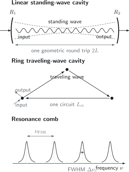
A linear cavity returns the field after a path of roughly $2L$ and can form a standing wave; a ring returns it after one circuit $L_{\mathrm{rt}}$ and can support traveling waves. In frequency space, adjacent longitudinal resonances are separated by $\nu_{\mathrm{FSR}}$, while one resonance has FWHM $\Delta\nu_c$.

The Round-Trip Eigenproblem

Let $\mathcal R(\omega)$ propagate a transverse, polarization-resolved field through one complete circuit, including mirrors, apertures, lenses, waveguides, and loss. A cavity mode satisfies

$$\mathcal R(\omega_\mu) u_\mu = \lambda_\mu(\omega_\mu) u_\mu.$$

For a passive cavity,

$$|\lambda_\mu|<1.$$

Its magnitude gives loss and its phase gives resonance. Writing

$$\lambda_\mu = \rho_\mu e^{i\Phi_{\mathrm{rt},\mu}},$$

the resonance condition is

$$\Phi_{\mathrm{rt},\mu} (\omega_{\mu q}) = 2\pi q, \qquad q\in\mathbb Z.$$

A scalar round-trip phase is justified only after the spatial and polarization eigenfunction has been identified. A plane wave at an arbitrary angle is not automatically a cavity mode.

Longitudinal Resonances

Free spectral range from group delay

For adjacent longitudinal resonances of the same transverse and polarization family,

$$\Phi_{\mathrm{rt}}(\omega_{q+1}) - \Phi_{\mathrm{rt}}(\omega_q) = 2\pi.$$

If the round-trip phase is smooth over one spacing,

$$\begin{aligned} \Delta\omega_{\mathrm{FSR}} &\simeq \frac{ 2\pi }{ d\Phi_{\mathrm{rt}}/d\omega }, \\ \nu_{\mathrm{FSR}} &\simeq \frac{1}{t_{\mathrm{rt}}}. \end{aligned}$$

This group-delay form is the safest general statement.

For an empty nondispersive linear cavity,

$$t_{\mathrm{rt}} = \frac{2n_gL}{c},$$

so

$$\nu_{\mathrm{FSR}} = \frac{c}{2n_gL}.$$

For a traveling-wave ring,

$$t_{\mathrm{rt}} = \frac{n_gL_{\mathrm{rt}}}{c}, \qquad \nu_{\mathrm{FSR}} = \frac{c}{n_gL_{\mathrm{rt}}}.$$

These formulas agree when the two structures have the same round-trip optical path.

Phase index versus group index

The resonance itself depends on phase accumulation. For a uniform linear cavity,

$$\Phi_{\mathrm{rt}} = \frac{2\omega n(\omega)L}{c} + \phi_{r1}(\omega) + \phi_{r2}(\omega).$$

Differentiation gives

$$\begin{aligned} t_{\mathrm{rt}} ={}& \frac{2n_gL}{c} \\ &+ \frac{d\phi_{r1}}{d\omega} + \frac{d\phi_{r2}}{d\omega}. \end{aligned}$$

Mirror-coating dispersion and intracavity material dispersion can therefore shift the FSR away from $c/(2nL)$. Near strong dispersion, adjacent spacings need not be uniform.

Length sensitivity

For a simple nondispersive cavity with fixed longitudinal index,

$$\frac{\delta\nu_q}{\nu_q} \simeq -\frac{\delta L_{\mathrm{opt}}}{L_{\mathrm{opt}}}.$$

This extreme conversion of fractional length noise into optical frequency noise is why high-finesse cavities are both excellent sensors and demanding frequency references.

Driven Fabry–Pérot Response

Sum the circulating fields

Choose a reference plane just inside the input mirror. Let $t_1$ be its field transmission and let $\rho$ be the magnitude of the remaining round-trip field multiplier. Successive returns form a geometric series:

$$\begin{aligned} E_{\mathrm{cav}} &= t_1E_{\mathrm{in}} \sum_{j=0}^{\infty} \left( \rho e^{i\Phi_{\mathrm{rt}}} \right)^j \\ &= \frac{ t_1E_{\mathrm{in}} }{ 1-\rho e^{i\Phi_{\mathrm{rt}}} }. \end{aligned}$$

The series converges for $\rho<1$. Its power denominator is

$$\begin{aligned} \left| 1-\rho e^{i\Phi_{\mathrm{rt}}} \right|^2 ={}& (1-\rho)^2 \\ &+ 4\rho \sin^2 \left( \frac{\Phi_{\mathrm{rt}}}{2} \right). \end{aligned}$$

Thus the circulating-power response is an Airy distribution:

$$\frac{ P_{\mathrm{cav}} }{ P_{\mathrm{in}} } = \frac{ T_1 }{ (1-\rho)^2 + 4\rho \sin^2 (\Phi_{\mathrm{rt}}/2) },$$

assuming perfect spatial and polarization mode matching at the chosen reference plane.

On resonance,

$$\left. \frac{ P_{\mathrm{cav}} }{ P_{\mathrm{in}} } \right|_{\mathrm{res}} = \frac{T_1}{(1-\rho)^2}.$$

High buildup therefore requires both low round-trip loss and deliberate matching of the input coupler to the other losses. A high-reflectivity input mirror alone does not guarantee efficient loading.

Airy coefficient and finesse

Write the normalized line shape as

$$\mathcal A_{\mathrm{cav}}(\phi) = \frac{1}{ 1+\mathscr F \sin^2(\phi/2) },$$

where

$$\mathscr F = \frac{4\rho}{(1-\rho)^2}$$

is the Airy coefficient. It is not the finesse.

When a conventional FWHM is defined, the exact phase-width result is

$$\mathcal F = \frac{ \pi }{ 2 \arcsin \left[ \dfrac{1-\rho}{2\sqrt{\rho}} \right] }.$$

In the high-finesse limit,

$$\mathcal F \simeq \frac{ \pi\sqrt{\rho} }{ 1-\rho }.$$

For a lossless symmetric two-mirror cavity with mirror power reflectivity $R$, the round-trip field survival is $\rho=R$, so

$$\mathcal F \simeq \frac{ \pi\sqrt R }{ 1-R }.$$

At low reflectivity, overlapping peaks, frequency-dependent coatings, and background paths make a single quoted finesse convention dependent. Fit the actual transfer function rather than forcing a high-finesse formula.

Loss, Lifetime, Linewidth, and Q

Round-trip survival

If the field is left undriven, the intracavity power is multiplied by

$$\mathcal S_{\mathrm{rt}} = \rho^2$$

each round trip. After $m=t/t_{\mathrm{rt}}$ circuits,

$$U(t) = U(0) \left( \mathcal S_{\mathrm{rt}} \right)^{t/t_{\mathrm{rt}}}.$$

Matching this to $U(0)e^{-\kappa t}$ gives

$$\kappa = -\frac{ \ln\mathcal S_{\mathrm{rt}} }{ t_{\mathrm{rt}} }.$$

For small round-trip power loss

$$\mathcal L_{\mathrm{rt}} = 1-\mathcal S_{\mathrm{rt}} \ll1,$$

one has

$$\kappa \simeq \frac{ \mathcal L_{\mathrm{rt}} }{ t_{\mathrm{rt}} }.$$

The loss should be decomposed as

$$\mathcal L_{\mathrm{rt}} \simeq \mathcal L_{\mathrm{out}} + \mathcal L_{\mathrm{abs}} + \mathcal L_{\mathrm{sc}} + \mathcal L_{\mathrm{diff}} + \mathcal L_{\mathrm{clip}},$$

when all contributions are small. The logarithmic form is preferable when they are not.

Lorentzian resonance

Near an isolated high-finesse resonance, the cavity behaves as a damped single mode. Its power line shape is Lorentzian with

$$\Delta\omega_c = \kappa, \qquad \Delta\nu_c = \frac{\kappa}{2\pi}.$$

Therefore

$$\begin{aligned} \tau_p &= \frac{1}{\kappa}, \\ Q &= \frac{\omega_c}{\kappa} = \frac{\nu_c}{\Delta\nu_c}, \\ \mathcal F &= \frac{\nu_{\mathrm{FSR}}}{\Delta\nu_c} \simeq \frac{2\pi}{ \kappa t_{\mathrm{rt}} }. \end{aligned}$$

The last relation assumes a well-isolated resonance and is asymptotically equivalent to the high-finesse Airy result.

Finesse and Q answer different questions

Finesse compares a linewidth with the spacing to the next longitudinal resonance. Quality factor compares that linewidth with the optical carrier frequency:

$$Q = \frac{\nu_c}{\nu_{\mathrm{FSR}}} \mathcal F.$$

The factor $\nu_c/\nu_{\mathrm{FSR}}$ is approximately the longitudinal mode order. Two cavities can have the same $Q$ but different finesse if their round-trip times differ.

The mean number of round trips during one photon lifetime is

$$\frac{\tau_p}{t_{\mathrm{rt}}} \simeq \frac{\mathcal F}{2\pi}.$$

It is not $\mathcal F$ itself.

Loss channels and escape efficiency

In a continuous-time model,

$$\kappa = \kappa_{\mathrm{out}} + \kappa_{\mathrm{other}}.$$

The probability that a stored photon exits through the desired port is

$$\eta_{\mathrm{esc}} = \frac{ \kappa_{\mathrm{out}} }{ \kappa }.$$

Increasing output coupling can improve extraction while lowering $Q$ and raising laser threshold. Input–Output Theory Overview owns the complex reflection and transmission amplitudes, critical coupling, and quantum noise entering through each port.

Spatial Stability

ABCD criterion

In one transverse plane, paraxial propagation through a complete round trip is represented by

$$M_{\mathrm{rt}} = \begin{pmatrix} A&B\\ C&D \end{pmatrix}, \qquad \det M_{\mathrm{rt}}=1.$$

Repeated rays remain bounded in the robust stable interior when

$$\left| \frac{A+D}{2} \right| < 1.$$

At equality, the cavity is marginal or degenerate. Finite apertures, misalignment, aberration, and diffraction then decide whether a useful low-loss mode exists.

Two spherical mirrors

For mirror radii of curvature $R_1$ and $R_2$ separated by $L$, define

$$g_1 = 1-\frac{L}{R_1}, \qquad g_2 = 1-\frac{L}{R_2}.$$

The standard stability interval is

$$0 < g_1g_2 < 1,$$

with $g_1g_2=0$ and $1$ marking idealized degenerate or marginal boundaries.

Examples:

Geometry	Parameters	Interpretation
plane–parallel	$R_1,R_2\to\infty$	$g_1g_2=1$, marginal
symmetric confocal	$R_1=R_2=L$	$g_1g_2=0$, degenerate boundary
symmetric concentric	$R_1=R_2=L/2$	$g_1g_2=1$, marginal
symmetric curved	$R_1=R_2=2L$	$g_1g_2=1/4$, stable interior

Sign conventions for $R_i$ vary with propagation direction. The final stability product must be computed with one consistent ray-matrix convention.

Transverse Modes

The fundamental Gaussian eigenmode

A stable spherical-mirror cavity supports a self-reproducing Gaussian mode whose complex beam parameter returns to itself under the round-trip ABCD map. For a symmetric cavity with

$$R_1=R_2=R,$$

the waist lies at the center and

$$z_R^2 = \frac{L}{2} \left( R-\frac{L}{2} \right).$$

The waist radius is

$$w_0^2 = \frac{\lambda z_R}{\pi},$$

and the mirror spot radius is

$$w_m = w_0 \sqrt{ 1+ \left( \frac{L}{2z_R} \right)^2 }.$$

These are paraxial, scalar, vacuum-wavelength formulas for a uniform medium. Astigmatism, thermal lenses, dielectric interfaces, and apertures modify the eigenmode.

Gouy phase and transverse spectrum

Hermite–Gaussian or Laguerre–Gaussian families acquire an additional Gouy phase. For an ideal stable two-mirror cavity,

$$\begin{aligned} \nu_{qmn} \simeq \nu_{\mathrm{FSR}} \bigg[ q &+ \frac{ m+n+1 }{ \pi } \\ &\times \arccos \sqrt{g_1g_2} \bigg]. \end{aligned}$$

The transverse order is $m+n$. The frequency shift per additional order is

$$\Delta\nu_\perp = \frac{ \nu_{\mathrm{FSR}} }{ \pi } \arccos \sqrt{g_1g_2}.$$

Near planar and near concentric limits, transverse families can become nearly degenerate modulo one FSR. Astigmatism separates horizontal and vertical Gouy phases. Birefringence and coating anisotropy can further split polarizations.

Frequency degeneracy does not imply identical loss. Aperture clipping, aberration, gain overlap, and mirror defects can discriminate strongly among transverse modes. Laser Modes develops their explicit field profiles, nodal structure, basis transformations, and nonlinear selection.

Mode Volume

For a lossless nondispersive cavity mode, an engineering mode volume referenced to the field maximum is

$$V_{\mathrm{cav}} = \frac{ \displaystyle \int \epsilon(\mathbf r) |\mathbf E(\mathbf r)|^2 d^3r }{ \displaystyle \max_{\mathbf r} \left[ \epsilon(\mathbf r) |\mathbf E(\mathbf r)|^2 \right] }.$$

For a fundamental standing-wave Gaussian mode with negligible waist variation over length $L$,

$$V_{\mathrm{cav}} \simeq \frac{ \pi w_0^2L }{4}.$$

The factor one half from transverse Gaussian integration and one half from longitudinal standing-wave averaging produce the factor one quarter.

For a traveling-wave ring with effective transverse area $A_{\mathrm{eff}}$,

$$V_{\mathrm{cav}} \sim A_{\mathrm{eff}}L_{\mathrm{rt}}.$$

These estimates are geometry tools, not universal quantization formulas. Dispersive, absorptive, open, nonlocal, or degenerate systems require the normalization discussed in Quantized Electromagnetic Modes.

Bridge to Cavity QED

Resonator design supplies two central scales:

• $Q$ controls photon storage and spectral selectivity;
• $V_{\mathrm{cav}}$ controls field concentration.

For a simple lossless mode, the electric field per quantum scales as

$$E_{\mathrm{zpf}} \propto \sqrt{ \frac{\omega_c}{ V_{\mathrm{cav}} } }.$$

Weak-coupling spontaneous-emission enhancement often scales schematically as $Q/V_{\mathrm{cav}}$, while coherent exchange also depends on dipole orientation, emitter position, detuning, and decoherence. A high-$Q$ cavity is not automatically a strong-coupling cavity.

Cavity QED develops the vacuum coupling $g$, cooperativity, dissipative polariton poles, and Purcell regime without conflating those quantities. Cavity QED Platforms compares open, fiber, nanophotonic, whispering-gallery, and microwave architectures and their calibration tradeoffs.

Worked Design Example

Consider an air-spaced symmetric linear cavity with

$$\begin{aligned} L &= 0.100\ \mathrm m, \\ R_1=R_2 &= 0.500\ \mathrm m, \\ \lambda &= 1064\ \mathrm{nm}, \\ \mathcal F &= 5.00\times10^4. \end{aligned}$$

The round-trip time and FSR are

$$\begin{aligned} t_{\mathrm{rt}} &= \frac{2L}{c} \simeq 6.671\times10^{-10}\ \mathrm s, \\ \nu_{\mathrm{FSR}} &= \frac{1}{t_{\mathrm{rt}}} \simeq 1.499\ \mathrm{GHz}. \end{aligned}$$

The cavity linewidth is

$$\Delta\nu_c = \frac{ \nu_{\mathrm{FSR}} }{ \mathcal F } \simeq 29.98\ \mathrm{kHz}.$$

Therefore

$$\begin{aligned} \kappa &= 2\pi\Delta\nu_c \simeq 1.884\times10^5\ \mathrm{s}^{-1}, \\ \tau_p &= \frac{1}{\kappa} \simeq 5.31\ \mu\mathrm s. \end{aligned}$$

The optical frequency and quality factor are

$$\begin{aligned} \nu_c &= \frac{c}{\lambda} \simeq 2.818\times10^{14}\ \mathrm{Hz}, \\ Q &= \frac{\nu_c}{\Delta\nu_c} \simeq 9.40\times10^9. \end{aligned}$$

The inferred round-trip power survival is

$$\begin{aligned} \mathcal S_{\mathrm{rt}} &= \exp \left( -\kappa t_{\mathrm{rt}} \right) \\ &\simeq 0.999874, \end{aligned}$$

corresponding to about $126$ parts per million total round-trip power loss. The photon lifetime contains

$$\frac{\tau_p}{t_{\mathrm{rt}}} \simeq 7.96\times10^3$$

round trips.

For the symmetric geometry,

$$g_1=g_2=0.800,$$

so the cavity is comfortably inside the stable region. The Rayleigh range and waist are

$$\begin{aligned} z_R &= \sqrt{ (0.050)(0.450) } = 0.150\ \mathrm m, \\ w_0 &= \sqrt{ \frac{ \lambda z_R }{\pi} } \simeq 225\ \mu\mathrm m. \end{aligned}$$

The standing-wave mode-volume estimate is

$$V_{\mathrm{cav}} \simeq \frac{\pi w_0^2L}{4} \simeq 3.99\ \mathrm{mm}^3.$$

Measuring a Cavity

Spectral scan

Scan laser frequency or cavity length and fit several resonances. This gives:

• FSR from peak spacing;
• linewidth from one isolated peak;
• finesse from their ratio;
• transverse and polarization splittings;
• mode-matching information from the distribution of peak areas.

A scan must be slow compared with the cavity response. Rapid sweeps can produce ringing and distort a static Airy or Lorentzian fit.

Cavity ringdown

Load the cavity, remove or rapidly detune the input, and fit transmitted power to

$$P(t) = P_0e^{-\kappa t} + P_{\mathrm{bg}}.$$

Ringdown measures total loss without requiring absolute calibration of circulating power. It does not by itself separate transmission, absorption, scattering, diffraction, and clipping.

Independent loss separation

Combine:

• calibrated mirror transmissions;
• reflected and transmitted resonant powers;
• cavity ringdown;
• mode-matching measurements;
• polarization-resolved spectra;
• aperture or alignment sweeps;
• wavelength-dependent coating data.

Loss separation is an inverse problem. Several channels can produce the same total linewidth.

A Reliable Cavity Workflow

1. Draw one complete round trip. Identify every propagation segment, reflection, coupler, and aperture.
2. Choose field or power coefficients. Do not mix $r$ with $R$.
3. Solve the spatial eigenproblem. Check stability and finite-aperture loss before applying a scalar resonance formula.
4. Compute phase and group delay separately. Phase sets resonance; group delay sets local FSR.
5. Inventory every loss channel. Distinguish useful output coupling from parasitic loss.
6. **Translate among $\rho$, $\mathcal S_{\mathrm{rt}}$, $\kappa$, $\Delta\nu_c$, $\mathcal F$, and $Q$ using definitions.
7. Check transverse and polarization spectra. A nearby mode can spoil a single-mode fit.
8. Include dispersion and thermal response when relevant. Coatings and materials can shift both resonance and FSR.
9. Validate with two observables. For example, compare spectral linewidth with ringdown time.
10. Propagate uncertainty. Length, frequency calibration, mode matching, and background offsets can dominate different inferred quantities.

Common Mistakes

Using one-way length as a ring round trip

A linear cavity has a $2L$ geometric round trip; a ring uses its full circuit once. Count the actual closed path.

Replacing group index by phase index in the FSR

Resonance phase involves $n$, but adjacent spacing involves $d\Phi_{\mathrm{rt}}/d\omega$ and therefore $n_g$ plus coating delay.

Calling the Airy coefficient finesse

$\mathscr F=4\rho/(1-\rho)^2$ appears inside the Airy denominator. $\mathcal F=\nu_{\mathrm{FSR}}/\Delta\nu_c$ is a frequency ratio.

Mixing amplitude and power reflectivity

For symmetric mirrors, $r=\sqrt R$ but the round-trip field multiplier is $r_1r_2=R$. Missing one square root creates large errors at high finesse.

Equating finesse with number of round trips

The energy lifetime contains approximately $\mathcal F/(2\pi)$ round trips under this linewidth convention.

Assuming stability guarantees low loss

The ABCD criterion only tests paraxial boundedness. Finite mirrors, aberrations, contamination, roughness, and mode mismatch still matter.

Treating high Q as small mode volume

$Q$ measures storage relative to carrier frequency. Mode volume measures spatial concentration. They are independent design axes.

Ignoring scan dynamics

A swept high-finesse cavity may ring. Fitting that transient as a static Airy peak biases the linewidth.

Exercises

1. Compare linear and ring FSRs

A vacuum linear cavity has mirror separation $L=0.30\ \mathrm m$. A vacuum ring has perimeter $L_{\mathrm{rt}}=0.60\ \mathrm m$. Find both free spectral ranges and explain the equality.

Solution

For the linear cavity,

$$\begin{aligned} \nu_{\mathrm{FSR,lin}} &= \frac{c}{2L} \\ &= \frac{2.998\times10^8}{0.60} \\ &\simeq 4.997\times10^8\ \mathrm{Hz}. \end{aligned}$$

For the ring,

$$\begin{aligned} \nu_{\mathrm{FSR,ring}} &= \frac{c}{L_{\mathrm{rt}}} \\ &= \frac{2.998\times10^8}{0.60} \\ &\simeq 4.997\times10^8\ \mathrm{Hz}. \end{aligned}$$

Both closed paths are $0.60\ \mathrm m$, so both round-trip group delays are the same. Geometry labels differ; the physical closed path does not.

2. Infer mirror reflectivity from finesse

A symmetric, otherwise lossless Fabry–Pérot cavity has $\mathcal F=3000$. Estimate each mirror power reflectivity using the high-finesse formula.

Solution

For $R\simeq1$,

$$\mathcal F \simeq \frac{\pi}{1-R}.$$

Therefore

$$\begin{aligned} 1-R &\simeq \frac{\pi}{3000} \\ &\simeq 1.047\times10^{-3}, \end{aligned}$$

so

$$R \simeq 0.998953.$$

The inferred transmission is about $1047$ parts per million per mirror. Any absorption, scattering, or diffraction would mean the actual mirror transmission is smaller than that all-loss attribution.

3. Convert a ringdown time

A cavity has $t_{\mathrm{rt}}=1.00\ \mathrm{ns}$ and measured photon lifetime $\tau_p=10.0\ \mu\mathrm s$. Find $\kappa$, round-trip power loss, and finesse.

Solution

The energy-decay rate is

$$\kappa = \frac{1}{\tau_p} = 1.00\times10^5\ \mathrm{s}^{-1}.$$

The exact round-trip survival is

$$\mathcal S_{\mathrm{rt}} = \exp(-\kappa t_{\mathrm{rt}}) = \exp(-10^{-4}),$$

so

$$\mathcal L_{\mathrm{rt}} \simeq 9.9995\times10^{-5},$$

or approximately $100$ parts per million.

Finally,

$$\mathcal F \simeq \frac{2\pi}{\kappa t_{\mathrm{rt}}} \simeq 6.283\times10^4.$$

4. Classify symmetric geometries

For a symmetric two-mirror cavity, evaluate $g_1g_2$ when $R/L$ is $\infty$, $2$, $1$, and $1/2$. Classify each case.

Solution

With $g=1-L/R$, the product is $g^2$:

$R/L$	$g$	$g^2$	Classification
$\infty$	$1$	$1$	plane–parallel marginal boundary
$2$	$1/2$	$1/4$	stable interior
$1$	$0$	$0$	confocal degenerate boundary
$1/2$	$-1$	$1$	concentric marginal boundary

Only $R=2L$ lies strictly inside $0<g_1g_2<1$.

5. Calculate a symmetric-cavity waist

A vacuum cavity has $L=50.0\ \mathrm{mm}$, $R_1=R_2=100\ \mathrm{mm}$, and $\lambda=780\ \mathrm{nm}$. Find $z_R$, $w_0$, and $w_m$.

Solution

The Rayleigh range is

$$\begin{aligned} z_R &= \sqrt{ \frac{L}{2} \left( R-\frac{L}{2} \right) } \\ &= \sqrt{ (0.0250)(0.0750) } \\ &\simeq 43.3\ \mathrm{mm}. \end{aligned}$$

Then

$$\begin{aligned} w_0 &= \sqrt{ \frac{\lambda z_R}{\pi} } \\ &\simeq 104\ \mu\mathrm m. \end{aligned}$$

At either mirror,

$$\begin{aligned} w_m &= w_0 \sqrt{ 1+ \left( \frac{L}{2z_R} \right)^2 } \\ &\simeq 120\ \mu\mathrm m. \end{aligned}$$

The spot radius is larger at the mirrors because the wavefront has propagated away from the central waist.

6. Find a transverse-mode spacing

A stable two-mirror cavity has $g_1g_2=0.81$ and $\nu_{\mathrm{FSR}}=1.50\ \mathrm{GHz}$. Find the frequency shift per unit increase in $m+n$.

Solution

Since

$$\sqrt{g_1g_2}=0.900,$$

the Gouy fraction is

$$\frac{ \arccos(0.900) }{\pi} \simeq 0.1436.$$

Therefore

$$\begin{aligned} \Delta\nu_\perp &\simeq (0.1436)(1.50\ \mathrm{GHz}) \\ &\simeq 215\ \mathrm{MHz}. \end{aligned}$$

Modes with the same $m+n$ remain degenerate in the ideal rotationally symmetric paraxial model.

7. Separate Q from finesse

Two cavities resonate at $\nu_c=3.00\times10^{14}\ \mathrm{Hz}$ and both have $Q=10^9$. Cavity A has FSR $1.00\ \mathrm{GHz}$; cavity B has FSR $10.0\ \mathrm{GHz}$. Find their linewidths and finesses.

Solution

Both linewidths are

$$\Delta\nu_c = \frac{\nu_c}{Q} = 3.00\times10^5\ \mathrm{Hz}.$$

For cavity A,

$$\mathcal F_A = \frac{1.00\times10^9}{3.00\times10^5} \simeq 3333.$$

For cavity B,

$$\mathcal F_B = \frac{1.00\times10^{10}}{3.00\times10^5} \simeq 3.33\times10^4.$$

Equal $Q$ fixes equal fractional linewidth at a common carrier frequency. The shorter-round-trip cavity has wider mode spacing and therefore larger finesse.

8. Diagnose inconsistent loss measurements

A spectral scan gives a cavity linewidth twice that inferred from a ringdown measurement. List checks that distinguish a real time dependence from a measurement artifact.

Solution

Check:

1. whether both analyses use power FWHM and energy-decay $\kappa$;
2. scan-frequency calibration and nonlinearity;
3. whether the scan is slow compared with $\tau_p$;
4. laser frequency noise and cavity length noise during the scan;
5. unresolved transverse or polarization doublets;
6. prompt-path interference that distorts the spectral line;
7. detector bandwidth, offset, and saturation;
8. whether ringdown subtraction removes a nondecaying background;
9. power-dependent absorption, thermal shift, or nonlinear loss;
10. whether the same mode and alignment were measured in both experiments.

If the disagreement changes with scan speed or probe power, the cavity is not being measured in the same linear stationary regime.

For a compact translation among finesse, $Q$, stored-energy decay, mode volume, threshold, and laser-output terminology, see Laser Nomenclature.

References

1. C. Fabry and A. Pérot, “Théorie et applications d’une nouvelle méthode de spectroscopie interférentielle,” Annales de Chimie et de Physique 16, 115–144 (1899).
2. A. G. Fox and T. Li, “Resonant Modes in a Maser Interferometer,” Bell System Technical Journal 40, 453–488 (1961).
3. G. D. Boyd and J. P. Gordon, “Confocal Multimode Resonator for Millimeter Through Optical Wavelength Masers,” Bell System Technical Journal 40, 489–508 (1961).
4. H. Kogelnik and T. Li, “Laser Beams and Resonators,” Applied Optics 5, 1550–1567 (1966).
5. Nur Ismail, C. C. Kores, D. Geskus, and M. Pollnau, “Fabry–Pérot Resonator: Spectral Line Shapes, Generic and Related Airy Distributions, Linewidths, Finesses, and Performance at Low or Frequency-Dependent Reflectivity,” Optics Express 24, 16366–16389 (2016).
6. A. O’Keefe and D. A. G. Deacon, “Cavity Ring-Down Optical Spectrometer for Absorption Measurements Using Pulsed Laser Sources,” Review of Scientific Instruments 59, 2544–2551 (1988).
7. K. An, C. Yang, R. R. Dasari, and M. S. Feld, “Cavity Ring-Down Technique and Its Application to the Measurement of Ultraslow Velocities,” Optics Letters 20, 1068–1070 (1995).
8. K. J. Vahala, “Optical Microcavities,” Nature 424, 839–846 (2003).
9. D. K. Armani, T. J. Kippenberg, S. M. Spillane, and K. J. Vahala, “Ultra-High-Q Toroid Microcavity on a Chip,” Nature 421, 925–928 (2003).
10. A. E. Siegman, Lasers, University Science Books (1986).
11. B. E. A. Saleh and M. C. Teich, Fundamentals of Photonics, 3rd ed., Wiley (2019).
12. O. Svelto, Principles of Lasers, 5th ed., Springer (2010), doi:10.1007/978-1-4419-1302-9.
13. A. Yariv and P. Yeh, Photonics: Optical Electronics in Modern Communications, 6th ed., Oxford University Press (2007).
14. H. Hunger et al., “A Fiber Fabry–Pérot Cavity with High Finesse,” New Journal of Physics 12, 065038 (2010).