Cavity QED Platforms

A cavity-QED platform places a quantum emitter in a selected resonator mode and engineers both the coherent interaction and the channels through which energy and information leave. The physical platform is not specified by a Jaynes–Cummings Hamiltonian alone. It also contains:

• a resonator geometry and polarization structure;
• an emitter source, trap, or trajectory;
• state preparation and frequency control;
• spatial and angular overlap with the vacuum field;
• useful ports and parasitic loss;
• cavity and emitter stabilization;
• a receiver chain; and
• a calibration model connecting detector records to intracavity dynamics.

The same symbols $g$, $\kappa$, and $\gamma$ can describe a neutral atom between macroscopic mirrors, an ion in a fiber cavity, a Rydberg atom crossing a superconducting microwave resonator, or an emitter near a photonic-crystal defect. The apparatus needed to realize and infer those rates is radically different in each case.

Canonical Scope

Cavity QED owns the universal single-emitter theory: vacuum-field normalization, $g(\mathbf r)$, cooperativity, lossy polariton poles, Purcell channeling, resonant extinction, and dispersive readout. Jaynes–Cummings Model owns the closed-model spectrum and excitation-exchange dynamics.

Optical Cavities owns free spectral range, finesse, quality factor, mode volume, Gaussian stability, Airy response, and ringdown. Input–Output Theory Overview owns empty-cavity port relations and receiver conventions. The open-system cavity-QED map owns conditional trajectories and continuous measurement records.

This page owns the physical implementation layer:

• optical resonator architectures and their experimental tradeoffs;
• microwave cavities probed by natural atoms;
• emitter loading, localization, cooling, and internal-state preparation;
• port, loss, mode-matching, and stabilization budgets;
• experimentally realized rather than ideal cooperativity;
• evidence required for strong-coupling and interface claims; and
• system-level applications and validation workflows.

Superconducting artificial atoms and their dispersive hardware stack belong to the separate circuit-QED overview.

Rate and Port Conventions

Throughout this page,

$$\kappa = \sum_j\kappa_j +\kappa_{\mathrm{int}}$$

is the cavity energy-decay rate. The intracavity photon number decays as $e^{-\kappa t}$, the field amplitude decays as $e^{-\kappa t/2}$, and

$$\frac{\kappa}{2\pi}$$

is the full width at half maximum of an isolated empty-cavity power resonance. The emitter population-decay rate outside the selected cavity channel is $\gamma$, while pure dephasing is $\gamma_\phi$. Its optical coherence rate is

$$\gamma_\perp = \frac{\gamma}{2} +\gamma_\phi.$$

The rate dictionary must be restated when comparing experiments. Some authors call the cavity field-amplitude decay rate $\kappa$, or use $\gamma$ for an atomic half width. Dimensionless numbers agree only after those definitions are translated.

For one designated output port,

$$\eta_{\mathrm{esc}} = \frac{\kappa_{\mathrm{use}}}{\kappa}$$

is the escape fraction conditional on a photon already occupying the cavity mode. It is not the mode-matching efficiency into the cavity, the emitter-to-cavity branching probability, propagation efficiency, or detector efficiency.

The Platform Is a Cascaded System

A useful cavity-QED experiment can be represented as

$$\text{source} \longrightarrow \text{emitter} \longleftrightarrow \text{cavity} \longrightarrow \text{port} \longrightarrow \text{receiver}.$$

Each arrow has its own state space and efficiency. For a generated photon, one possible end-to-end accounting is

$$P_{\mathrm{click}} = P_{\mathrm{prep}} P_{\mathrm{emit}} \beta_{\mathrm{cav}} \eta_{\mathrm{esc}} \eta_{\mathrm{path}} \eta_{\mathrm{det}},$$

where the factors are conditional in sequence:

• $P_{\mathrm{prep}}$ prepares the emitter and motional state;
• $P_{\mathrm{emit}}$ completes the intended control protocol;
• $\beta_{\mathrm{cav}}$ sends the photon into the selected cavity mode;
• $\eta_{\mathrm{esc}}$ sends it through the useful port;
• $\eta_{\mathrm{path}}$ transmits it through filters, fibers, and optics; and
• $\eta_{\mathrm{det}}$ converts the arriving photon into an accepted record.

The product is a bookkeeping model, not a universal independence assumption. Spectral mismatch can correlate emission, escape, and path transmission; detector dead time can correlate successive trials.

Optical Cavity Platforms

Open Fabry–Pérot cavities

Two opposing mirrors form the most direct optical cavity-QED architecture. Its strengths are:

• an open mode volume that can be loaded with neutral atoms, ions, molecules, ensembles, or solid-state samples;
• well-understood Gaussian modes and polarization control;
• independent input and output ports;
• access for trapping, cooling, and control beams; and
• high finesse with low-loss dielectric coatings.

For a linear cavity of optical length $L_{\mathrm{opt}}$,

$$\nu_{\mathrm{FSR}} \approx \frac{c}{2L_{\mathrm{opt}}},$$

and, for an isolated high-finesse resonance,

$$\frac{\kappa}{2\pi} = \delta\nu_{\mathrm{cav}} \approx \frac{\nu_{\mathrm{FSR}}}{\mathcal F}.$$

The approximate standing-wave mode volume

$$V \sim \frac{\pi w_0^2L_{\mathrm{phys}}}{4}$$

shows why short cavities and small waists raise the vacuum field. The exact definition, refractive-index weighting, and open-mode corrections remain on the canonical cavity pages.

Open access brings engineering costs:

• cavity length noise directly becomes detuning noise;
• mirrors constrain optical access and trap geometry;
• intracavity traps can shift the emitter and cavity coatings can charge;
• transverse modes can approach the working resonance;
• atomic motion samples the standing wave; and
• mirror transmission must be balanced against absorption and scatter.

High finesse is useful only if the cavity can be locked without injecting unacceptable photons, heating, or differential Stark shifts during the quantum sequence.

Fiber Fabry–Pérot cavities

Laser-machined concave structures on fiber facets can produce short cavities with small waists while coupling naturally to fiber modes. They are attractive when compactness and a large $g$ matter.

Their practical ledger includes:

• overlap between the cavity eigenmode and the fiber guided mode;
• asymmetric mirror transmissions chosen for a preferred port;
• coating loss and scattering on small curved surfaces;
• birefringence and polarization-mode splitting;
• dielectric charging near trapped ions or atoms;
• limited side access;
• mechanical and thermal stability of the fiber mounts; and
• contamination or damage under vacuum.

The small geometric mode volume is a maximum-coupling statement. Realized performance still depends on placing and cooling the emitter at the correct standing-wave antinode.

Photonic-crystal and nanobeam cavities

Photonic-band-gap defects can confine optical fields to wavelength-scale volumes and route output directly into a waveguide. This can produce a large vacuum field without extreme photon storage time.

Important departures from an open Fabry–Pérot cavity are:

• the emitter samples a strongly varying near field;
• polarization can vary within the mode;
• surfaces are close enough to create Casimir–Polder forces, charging, heating, or spectral shifts;
• fabrication disorder changes resonance frequency, quality factor, and port coupling;
• the cavity may be one-sided only after waveguide and intrinsic losses are separated; and
• quasinormal-mode normalization may be needed in an open or dispersive structure.

For trapped atoms, the nanostructure must be integrated with a stable near-surface trap. For solid-state emitters, implantation position, dipole orientation, spectral diffusion, phonon sidebands, and inhomogeneous fabrication spread replace atomic loading as dominant challenges.

Whispering-gallery and ring resonators

Total internal reflection confines traveling-wave modes around a dielectric boundary. Atoms or other emitters couple to the evanescent field. Advantages include high quality factor, small effective mode volume, and natural waveguide or fiber coupling.

Real devices often support clockwise and counterclockwise modes. Surface roughness couples them and produces standing-wave doublets. An apparent spectral splitting can therefore arise from cavity backscattering before an emitter is introduced. Empty-cavity polarization and direction-mode spectra are essential controls.

Architecture comparison

Optical architecture	Principal strength	Typical dominant constraint	Essential calibration
Macroscopic Fabry–Pérot	Open access and high finesse	Length noise and moderate mode volume	Ringdown, waist, mirror transmissions
Fiber Fabry–Pérot	Small volume and direct fiber interface	Birefringence, access, coating loss	Fiber mode matching and polarization splitting
Photonic crystal	Wavelength-scale volume and integration	Surface physics and fabrication disorder	Local field map and waveguide loss
Whispering-gallery or ring	High $Q$ with evanescent access	Counterpropagating-mode coupling	Empty-cavity doublet and external coupling

No row is uniformly best. The right objective may be coherent swaps, single-pass extinction, high photon extraction, long emitter coherence, parallel fabrication, or optical-network compatibility.

Microwave Cavities with Natural Atoms

Why Rydberg atoms compensate for long wavelength

Microwave modes occupy much larger physical volumes than optical modes, so their zero-point electric field is smaller. Highly excited Rydberg atoms compensate through:

• electric-dipole matrix elements that grow strongly with principal quantum number;
• long radiative lifetimes;
• adjacent transitions in the microwave domain; and
• state-selective field ionization after the atom leaves the cavity.

In traditional microwave cavity QED, circular Rydberg atoms cross a superconducting cavity one by one. Their coupling is time dependent,

$$g(t) = g_0 u[\mathbf r(t)] C_{\mathrm{ang}}(t),$$

and the interaction pulse area is controlled by velocity, trajectory, Stark tuning, and the spatial mode.

The atom is both quantum system and probe. Ramsey zones before and after the cavity can convert a photon-number-dependent phase into an atomic-state probability without absorbing the photon.

Thermal photons

The mean thermal occupation of a mode at angular frequency $\omega_c$ and temperature $T$ is

$$\bar n_{\mathrm{th}} = \frac{1}{ \exp(\hbar\omega_c/k_BT)-1 }.$$

At optical frequency, room-temperature thermal occupation is negligible. At microwave frequency it is an experimental variable.

For

$$\frac{\omega_c}{2\pi} = 51\,\mathrm{GHz},$$

the quantum energy corresponds to

$$\frac{\hbar\omega_c}{k_B} = 2.45\,\mathrm K.$$

Therefore,

$$\bar n_{\mathrm{th}} \approx \begin{cases} 0.049, & T=0.80\,\mathrm K,\\ 1.19, & T=4.0\,\mathrm K,\\ 122, & T=300\,\mathrm K. \end{cases}$$

A cryogenic enclosure, low-emissivity apertures, and thermal filtering are part of state preparation. Measuring the empty-cavity photon statistics is stronger evidence than inferring temperature from a cryostat sensor.

Storage, transit, and detection

Superconducting microwave cavities can store photons much longer than an atom’s transit time. This enables repeated nondemolition probes of the same field and feedback that responds to individual quantum jumps.

The platform must separately characterize:

• cavity energy lifetime and residual thermal occupation;
• atomic velocity and trajectory distribution;
• preparation of one Rydberg state;
• Ramsey-zone phase and contrast;
• dc Stark shifts and stray electric fields;
• atom-counting and state-selective-ionization errors; and
• latency and actuator calibration for feedback.

This natural-atom architecture differs from circuit QED, where a fabricated artificial atom is permanently integrated with a microwave resonator.

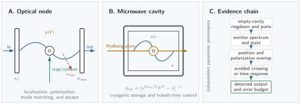
Physical cavity QED has more layers than the three-rate model. A: an optical node combines emitter localization, useful-port coupling, and parasitic loss. B: a flying Rydberg atom samples a cryogenic microwave mode whose thermal occupation must be measured. C: strong-coupling or interface claims become persuasive when empty-cavity, emitter, overlap, coupled-response, and receiver calibrations form one independent evidence chain.

Realizing Atom–Cavity Coupling

Maximum versus realized coupling

For a chosen transition, write

$$g(\mathbf r) = g_0 u(\mathbf r) C_{\mathrm{pol}} C_{\mathrm{int}},$$

where:

• $g_0$ is the maximum coupling for a reference dipole at the field maximum;
• $u(\mathbf r)$ is the complex spatial mode normalized to unit maximum;
• $C_{\mathrm{pol}}$ is the projection onto local polarization; and
• $C_{\mathrm{int}}$ contains the angular-momentum matrix element relative to the reference transition.

For a moving emitter, spectroscopy often depends on

$$\langle|g|^2\rangle = g_0^2 \left\langle |u(\mathbf r)|^2 |C_{\mathrm{pol}}|^2 |C_{\mathrm{int}}|^2 \right\rangle.$$

Replacing the distribution by one fitted $g$ can hide correlations between position, internal state, and probe-induced motion.

Standing-wave localization

Near a Fabry–Pérot antinode, a Gaussian standing-wave field may be modeled as

$$u(r,z) = \exp\left(-\frac{r^2}{w_0^2}\right) \cos(kz).$$

For a Gaussian axial position distribution of variance $\sigma_z^2$ centered at $z_0$,

$$\left\langle \cos^2(kz) \right\rangle = \frac12 \left[ 1 + e^{-2k^2\sigma_z^2} \cos(2kz_0) \right].$$

The same mean coupling can arise from a tightly localized atom away from an antinode or a broadly distributed atom centered at one. Sideband spectra, trap-frequency measurements, and position-dependent cavity transmission help distinguish them.

Trapping and cooling inside the mode

Neutral atoms may be delivered by a fountain, conveyor lattice, moving optical tweezer, or loading from a magneto-optical trap. Ions can be held by electrodes while a cavity is positioned around the radio-frequency trap. Flying atomic beams trade long interaction time for simple replenishment.

Intracavity trapping introduces coupled design constraints:

• the trap should localize the emitter where $|g|$ is large;
• differential Stark shifts should not destroy resonance or qubit coherence;
• trap light should not populate or heat the cavity mode;
• cavity cooling or sideband cooling should remove recoil heating;
• the cavity lock should remain stable when control beams switch; and
• a lost emitter should be distinguished from a state change.

The Optical Tweezers and Ion Traps pages own the corresponding confinement principles.

Multilevel structure

A real alkali atom, ion, molecule, quantum dot, or defect is not exactly a two-level emitter. Cavity polarization and magnetic field select among Zeeman or hyperfine transitions. Off-resonant states can produce:

• additional dispersive shifts;
• Raman scattering and optical pumping;
• polarization rotation;
• dark states;
• leakage outside the qubit manifold; and
• unequal couplings to nominally degenerate cavity polarizations.

An effective two-level model should be checked by varying magnetic field, probe polarization, detuning, and control-state preparation. A fitted $\gamma$ should not silently absorb optical pumping into dark states.

Collective coupling

For $N$ emitters in the weak-excitation limit, the bright collective coupling is

$$G = \sqrt{ \sum_{i=1}^{N} |g_i|^2 }.$$

For identical couplings, $G=\sqrt N\,g$. In an ensemble, however, atom number and coupling distribution fluctuate. A reported collective cooperativity therefore requires:

• atom-number or optical-depth calibration;
• spatial overlap with the cavity mode;
• internal-state population;
• inhomogeneous detuning and Doppler width;
• saturation checks; and
• evidence that dark collective modes do not dominate later dynamics.

Port and Loss Engineering

Useful and parasitic channels

The cavity decay ledger is

$$\kappa = \kappa_1 +\kappa_2 +\kappa_{\mathrm{wg}} +\kappa_{\mathrm{abs}} +\kappa_{\mathrm{sc}} +\cdots.$$

Only selected terms are useful for a given task. A reflection interface may want one dominant input–output port. A transmission experiment needs two ports. A network node may sacrifice storage time to make $\kappa_{\mathrm{use}}/\kappa$ large.

The design trade is explicit:

• decreasing useful transmission can raise finesse and $Q$;
• increasing useful transmission can improve escape and bandwidth;
• intrinsic loss reduces both storage and collection;
• port asymmetry changes the reflected phase and impedance condition.

The loaded linewidth alone cannot separate these contributions. Combine ringdown with calibrated reflection and transmission, or use independent mirror and waveguide characterization.

Mode matching

Let $\eta_{\mathrm{mm}}$ be the fraction of incident power in the selected spatial, polarization, and frequency mode. Promptly reflected light from orthogonal modes can interfere with cavity leakage at the detector. A power dip is therefore not a direct measurement of intracavity absorption.

Useful checks include:

• scanning an empty cavity while measuring complex reflection;
• imaging transmitted transverse modes;
• reversing polarization and propagation direction;
• varying the spatial mode-matching optics;
• separating promptly reflected and delayed fields in time; and
• confirming power-independent behavior below saturation.

Frequency stabilization

Define detunings

$$\Delta_c = \omega_p-\omega_c, \qquad \Delta_a = \omega_p-\omega_a.$$

Technical fluctuations give distributions of both variables. Cavity length noise, laser noise, magnetic-field noise, ac Stark shifts, and emitter motion can broaden a spectrum in different ways.

A lock system should report:

• in-loop and, when possible, out-of-loop frequency noise;
• bandwidth and residual drift;
• lock-beam detuning, polarization, and power;
• switching transients into the science window;
• conversion from error signal to physical detuning; and
• correlations between lock state and accepted trials.

An apparently broad atomic linewidth can be cavity jitter, and an apparently broad cavity can be scan nonlinearity.

Cooperativity as a Platform Metric

Ideal and effective values

With negligible pure dephasing, use

$$C_0 = \frac{4g_0^2}{\kappa\gamma}$$

for maximum single-emitter cooperativity. A motion- and state-averaged value is

$$C_{\mathrm{eff}} = \frac{ 4\langle|g|^2\rangle }{ \kappa\gamma }.$$

If pure dephasing matters, the weak-probe response is instead organized by

$$C_\perp = \frac{ 2\langle|g|^2\rangle }{ \kappa\gamma_\perp }.$$

These values answer a channel-competition question. They do not alone establish resolved coherent exchange.

Geometry is not the whole metric

For an idealized optical transition and cavity, one often summarizes design as “large $Q/V$.” The realized cooperativity also depends on:

• branching ratio of the selected transition;
• Debye–Waller or zero-phonon fraction for solid-state emitters;
• angular-momentum coefficient;
• position and polarization overlap;
• spectral diffusion and pure dephasing;
• atom number and state purity; and
• additional cavity modes.

Publishing both $C_0$ and $C_{\mathrm{eff}}$, with the reduction factors listed, prevents a simulated field maximum from being mistaken for measured performance.

Worked optical-cavity audit

Consider a linear cavity with

$$\begin{aligned} L &= 200\,\mu\mathrm m, \\ \mathcal F &= 5.00\times10^4, \\ \lambda &= 780\,\mathrm{nm}. \end{aligned}$$

Its free spectral range is

$$\nu_{\mathrm{FSR}} = \frac{c}{2L} = 7.49\times10^{11}\,\mathrm{Hz}.$$

The empty-cavity full width is

$$\frac{\kappa}{2\pi} = \frac{\nu_{\mathrm{FSR}}}{\mathcal F} = 15.0\,\mathrm{MHz}.$$

Thus the energy lifetime is

$$\tau_E = \frac{1}{\kappa} = 10.6\,\mathrm{ns},$$

while the field-amplitude $1/e$ time is $2/\kappa=21.2\,\mathrm{ns}$.

Suppose independent spectroscopy gives

$$\frac{g_0}{2\pi} = 25.0\,\mathrm{MHz}, \qquad \frac{\gamma}{2\pi} = 6.0\,\mathrm{MHz}.$$

Then

$$\begin{aligned} C_0 &= \frac{ 4(25.0)^2 }{ (15.0)(6.0) } \\ &= 27.8. \end{aligned}$$

If motion and internal-state preparation reduce $\sqrt{\langle|g|^2\rangle}$ to $0.70g_0$, then

$$C_{\mathrm{eff}} = (0.70)^2C_0 = 13.6.$$

Both are high-cooperativity values. A strong-coupling claim still requires a comparison of $g$ with the dissipative pole widths and evidence that the observed doublet belongs to one emitter and one cavity mode.

Strong Coupling as an Evidence Claim

Rate comparison

Informally, strong coupling requires coherent exchange to outpace the relevant cavity and emitter coherence losses:

$$g \gtrsim \kappa, \gamma_\perp$$

up to the chosen quantitative criterion. Exact resolvability depends on the complex polariton poles, drive port, detection quadrature, and detuning. The canonical Cavity QED page derives that response.

High cooperativity can occur in a bad-cavity regime,

$$\kappa \gg g \gg \gamma,$$

because $C$ depends on $g^2/(\kappa\gamma)$. Such a platform may be excellent for channeling and readout without supporting several coherent swaps.

Spectral evidence

A persuasive vacuum-Rabi measurement:

1. calibrates the empty-cavity resonance and polarization modes;
2. prepares a verified single emitter;
3. tunes emitter detuning across the cavity;
4. resolves two branches with an avoided crossing near resonance;
5. fits complex amplitudes or multiple ports when possible;
6. constrains $g$, $\kappa$, and $\gamma_\perp$ independently;
7. tests probe-power dependence below and through saturation; and
8. rules out classical cavity doublets, multiple emitters, and prompt-path interference.

Two peaks at one detuning are not enough. An empty-cavity birefringence doublet or whispering-gallery backscattering can look similar.

Time-domain evidence

Time-domain exchange can be even more direct. Prepare one excitation, tune atom and cavity into resonance for a controlled interval, and measure the oscillatory transfer. The analysis must include:

• finite pulse rise time;
• detuning jitter;
• cavity leakage during the interaction;
• spontaneous emission;
• motion-dependent $g(t)$;
• state-preparation and readout errors; and
• postselection on emitter survival.

Oscillations establish coherent dynamics only when classical beating among multiple frequencies has been excluded.

Applications

Deterministic or heralded single-photon sources

A cavity can direct spontaneous emission into a selected spatial mode, while Raman or adiabatic protocols control photon timing and polarization. A source specification should include:

• generation probability per trigger;
• output-mode and spectral purity;
• $g^{(2)}(0)$ or another multiphoton metric;
• indistinguishability from two-photon interference;
• repetition rate and dead time;
• frequency drift;
• fiber-coupled and detector-independent efficiency; and
• the treatment of lost-emitter trials.

Antibunching alone does not establish high brightness or indistinguishability.

Quantum-network nodes

An atom or ion supplies a long-lived local state, while the cavity maps that state to a propagating photon. The node must send, receive, store, and read out with compatible modes.

Network performance depends on more than local cooperativity:

$$P_{\mathrm{link}} \sim P_A P_B \eta_{\mathrm{ch}} \eta_{\mathrm{BSM}},$$

for a schematic two-node heralding protocol. Here $P_A$ and $P_B$ are node-level photon or memory efficiencies, $\eta_{\mathrm{ch}}$ is channel transmission, and $\eta_{\mathrm{BSM}}$ summarizes the relevant interference and detection success.

Photon waveform, frequency, polarization, timing, and indistinguishability must match between nodes. A high local extraction rate cannot compensate for poor remote interference.

Nondestructive detection and readout

A cavity converts a state-dependent susceptibility into a large reflected phase or transmitted intensity change. Applications include:

• detecting an atom without many free-space scattered photons;
• reading a qubit state;
• detecting an optical photon nondestructively;
• monitoring cavity photon number with dispersive atoms; and
• continuous feedback.

The measurement information and backaction are linked. Report spontaneous scattering, Raman flips, dephasing, loss, and detector efficiency together with assignment fidelity.

Gates and quantum nonlinear optics

An emitter can make the cavity response depend on one photon or one internal state. This supports atom–photon gates, photon routing, conditional phases, and photon blockade.

A nonlinear classical transmission curve is not by itself a quantum gate. Gate evidence requires:

• a defined computational mode and Hilbert space;
• truth-table or process information;
• phase coherence, not only intensity contrast;
• leakage and loss accounting;
• multiphoton contamination;
• mode distortion; and
• an appropriate fidelity benchmark.

Cavity cooling

The cavity can preferentially scatter photons that remove motional energy. The cooling limit depends on cavity linewidth, detuning, recoil geometry, trap frequencies, and technical noise. The cavity may cool an emitter even when a closed free-space optical cycle is unavailable.

Cooling evidence separates:

• damping rate from trap loss;
• final temperature or mode occupation;
• cavity-induced diffusion;
• free-space scattering;
• position dependence; and
• survival-conditioned bias.

Collective measurement and many-body physics

An ensemble coupled to one mode acquires collective measurement and cavity-mediated interaction channels. These enable spin squeezing, superradiance, long-range interactions, and self-organization.

The cavity mode imposes a spatial interaction kernel. Claims about an all-to-all collective model must bound:

• coupling inhomogeneity;
• multimode structure;
• atom loss and motion;
• spontaneous emission;
• finite cavity response time; and
• correlations introduced by conditioning on detected light.

Calibration and Validation Ledger

Layer	Parameter	Independent measurement	Failure if omitted
Empty cavity	$\omega_c$, $\kappa$, $\kappa_j$	Ringdown plus complex reflection/transmission	Port loss absorbed into fitted $g$
Spatial mode	Waist, antinode, polarization	Mode imaging, transverse spectrum, position scan	$g_0$ confused with realized $g$
Emitter	$\omega_a$, $\gamma$, $\gamma_\phi$	Free-space or far-detuned spectroscopy	Cavity jitter called emitter dephasing
Internal state	Population and dipole matrix element	State-selective spectroscopy	Optical pumping hidden in linewidth
Motion	$\sigma_r$, $\sigma_z$, mode occupation	Sidebands, trap frequencies, imaging	Coupling distribution ignored
Coupled response	$g$ and detuning	Avoided crossing, time-domain exchange	Classical doublet misidentified
Ports	$\eta_{\mathrm{esc}}$, $\eta_{\mathrm{mm}}$	Calibrated input/output powers	Intracavity branching called collection
Receiver	$\eta_{\mathrm{det}}$, dark counts, bandwidth	Calibrated light and null trials	Detector artifact called quantum signal
End to end	Success, erasure, and conditional fidelity	Tagged trial ledger	Postselection hidden

Minimal reproducibility package

A mature platform result reports:

• the linewidth convention and equations used in the fit;
• empty-cavity ringdown and port decomposition;
• cavity mode and polarization structure;
• emitter number, internal state, motion, and survival;
• independent detuning and frequency-noise calibrations;
• maximum and realized $g$;
• probe-power and saturation dependence;
• receiver efficiency and bandwidth;
• all conditional postselection;
• uncertainty and covariance for derived cooperativity; and
• raw observables that test at least one alternative explanation.

Common Mistakes

“High Q means strong coupling”

$Q$ controls storage, while $g$ also depends on mode volume, transition dipole, position, polarization, and internal state. Emitter decoherence is a separate scale.

“Small mode volume guarantees large usable g”

Only at the field maximum and correct polarization. Near-surface trapping, motion, spectral diffusion, and fabrication disorder can dominate.

“Cooperativity above one proves coherent swaps”

High-cooperativity bad-cavity systems efficiently route emission but may be overdamped in time.

“The cavity linewidth tells me the useful output”

The linewidth is the sum of useful ports and intrinsic loss. Escape efficiency requires their decomposition.

“A transmission doublet is vacuum Rabi splitting”

Polarization modes, backscattering, multiple emitters, scan artifacts, and prompt-path interference can also produce two features.

“The fitted g is a geometric constant”

It can be an average over motion, Zeeman states, occupancy, and technical drift. State which distribution the fit represents.

“Microwave cavities are automatically in vacuum”

Thermal occupation is appreciable unless $\hbar\omega_c\gg k_BT$ and the mode is shielded from warmer radiation.

“Detected photon probability is cavity efficiency”

Preparation, emission, branching, escape, propagation, and detection are distinct factors.

Exercises

1. Linewidth and lifetime conventions

A linear optical cavity has length $L=300\,\mu\mathrm m$ and finesse $\mathcal F=6.0\times10^4$.

1. Find the free spectral range.
2. Find $\kappa/(2\pi)$ under this page’s convention.
3. Find the intracavity energy and field-amplitude $1/e$ times.

Solution

The free spectral range is

$$\nu_{\mathrm{FSR}} = \frac{c}{2L} = 4.997\times10^{11}\,\mathrm{Hz}.$$

The power-resonance full width is

$$\frac{\kappa}{2\pi} = \frac{\nu_{\mathrm{FSR}}}{\mathcal F} = 8.33\,\mathrm{MHz}.$$

Thus

$$\kappa = 2\pi(8.33\times10^6)\,\mathrm{s^{-1}} = 5.23\times10^7\,\mathrm{s^{-1}}.$$

The energy lifetime is

$$\tau_E = \frac{1}{\kappa} = 19.1\,\mathrm{ns}.$$

Since field amplitude decays at $\kappa/2$,

$$\tau_A = \frac{2}{\kappa} = 38.2\,\mathrm{ns}.$$

Calling $1/\kappa$ the amplitude lifetime would create a factor-of-two error.

2. Motion-averaged coupling

An atom is centered at an antinode of

$$u(r,z) = e^{-r^2/w_0^2}\cos(kz).$$

Its axial position is Gaussian with $k\sigma_z=0.30$. Each transverse Cartesian coordinate is Gaussian with $\sigma_r/w_0=0.10$. Internal-state and polarization overlap are ideal. Find $\langle|g|^2\rangle/g_0^2$ and $g_{\mathrm{rms}}/g_0$.

Solution

At an antinode,

$$\left\langle \cos^2(kz) \right\rangle = \frac{ 1+e^{-2k^2\sigma_z^2} }{2} = \frac{1+e^{-0.18}}{2} = 0.918.$$

For two independent transverse Gaussian coordinates,

$$\left\langle e^{-2r^2/w_0^2} \right\rangle = \frac{1}{ 1+4\sigma_r^2/w_0^2 } = \frac{1}{1.04} = 0.962.$$

Therefore

$$\frac{ \langle|g|^2\rangle }{ g_0^2 } = (0.918)(0.962) = 0.883,$$

and

$$\frac{g_{\mathrm{rms}}}{g_0} = \sqrt{0.883} = 0.940.$$

The average amplitude $\langle g\rangle$ is not generally the quantity that sets weak-probe cooperativity; the squared coupling enters.

3. High cooperativity without strong coupling

A platform has

$$\frac{g}{2\pi} = 10\,\mathrm{MHz}, \quad \frac{\kappa}{2\pi} = 100\,\mathrm{MHz}, \quad \frac{\gamma}{2\pi} = 0.10\,\mathrm{MHz},$$

with negligible pure dephasing. Find $C$ and classify the regime.

Solution

Common factors of $2\pi$ cancel:

$$C = \frac{4g^2}{\kappa\gamma} = \frac{ 4(10)^2 }{ (100)(0.10) } = 40.$$

The cooperativity is high, so cavity-mediated emission can dominate free-space decay. However,

$$\kappa = 10g,$$

so a cavity excitation leaks much faster than a coherent exchange period. This is a high-cooperativity bad-cavity or Purcell regime, not unambiguous strong coupling.

4. From cavity emission to a click

In a simple high-cooperativity emission model, take

$$\beta_{\mathrm{cav}} = \frac{C}{1+C}.$$

For $C=19$, a useful-port fraction $\eta_{\mathrm{esc}}=0.75$, path transmission $\eta_{\mathrm{path}}=0.60$, and detector efficiency $\eta_{\mathrm{det}}=0.80$:

1. find the click probability conditional on successful emitter preparation and emission;
2. identify which factor should be improved first if its relative cost is comparable.

Solution

The cavity branching estimate is

$$\beta_{\mathrm{cav}} = \frac{19}{20} = 0.95.$$

The conditional click probability is

$$\begin{aligned} P_{\mathrm{click|emit}} &= (0.95)(0.75)(0.60)(0.80) \\ &= 0.342. \end{aligned}$$

Only 34.2% of successful emission trials produce a click. The smallest factor is path transmission, so a comparable fractional improvement there usually gives the largest absolute benefit. Raising $C$ further has limited leverage because $\beta_{\mathrm{cav}}$ is already 0.95.

The formula ignores spectral mismatch, detector dead time, and correlations between escape and path filtering.

5. Microwave thermal occupation

For a $51\,\mathrm{GHz}$ cavity:

1. calculate $\hbar\omega_c/k_B$;
2. find $\bar n_{\mathrm{th}}$ at $0.50\,\mathrm K$ and $1.0\,\mathrm K$;
3. find the temperature required for $\bar n_{\mathrm{th}}=0.01$.

Solution

Since $\hbar\omega_c=h\nu_c$,

$$\frac{\hbar\omega_c}{k_B} = \frac{h(51\times10^9)}{k_B} = 2.45\,\mathrm K.$$

At $0.50\,\mathrm K$,

$$\bar n_{\mathrm{th}} = \frac{1}{e^{2.45/0.50}-1} = 7.5\times10^{-3}.$$

At $1.0\,\mathrm K$,

$$\bar n_{\mathrm{th}} = \frac{1}{e^{2.45}-1} = 9.45\times10^{-2}.$$

For a target $\bar n$,

$$\frac{\hbar\omega_c}{k_BT} = \ln\left(1+\frac{1}{\bar n}\right).$$

Thus

$$T = \frac{2.45\,\mathrm K}{\ln101} = 0.530\,\mathrm K.$$

The cavity can still see excess photons from warmer apertures or technical injection even when the local cryostat temperature satisfies this estimate.

6. Port redesign

A cavity has

$$\kappa_{\mathrm{use}} = 2\pi(6\,\mathrm{MHz}), \quad \kappa_{\mathrm{other}} = 2\pi(2\,\mathrm{MHz}), \quad \kappa_{\mathrm{int}} = 2\pi(2\,\mathrm{MHz}).$$

The emitter coupling and decay are

$$\frac{g}{2\pi} = 12\,\mathrm{MHz}, \qquad \frac{\gamma}{2\pi} = 3\,\mathrm{MHz}.$$

Find $\eta_{\mathrm{esc}}$ and $C$. Then double $\kappa_{\mathrm{use}}$ while leaving all other quantities unchanged. Recompute both and explain the trade.

Solution

Initially,

$$\frac{\kappa}{2\pi} = 6+2+2 = 10\,\mathrm{MHz},$$

so

$$\eta_{\mathrm{esc}} = \frac{6}{10} = 0.60.$$

The cooperativity is

$$C = \frac{4(12)^2}{(10)(3)} = 19.2.$$

After doubling the useful coupling,

$$\frac{\kappa'}{2\pi} = 12+2+2 = 16\,\mathrm{MHz},$$

and

$$\eta_{\mathrm{esc}}' = \frac{12}{16} = 0.75.$$

However,

$$C' = \frac{4(12)^2}{(16)(3)} = 12.0.$$

The useful escape fraction improves while storage and cooperativity fall. The best choice depends on whether the protocol is limited by internal channeling, output extraction, bandwidth, or coherent exchange.

7. Audit a spectral doublet

A paper shows two transmission peaks when one atom is nominally resonant with a cavity and calls them vacuum Rabi splitting. List the minimum additional measurements needed to make that interpretation persuasive.

Solution

A defensible audit includes:

1. an empty-cavity spectrum resolving polarization, transverse, and counterpropagating-mode splittings;
2. independent ringdown or linewidth measurement;
3. verified single-emitter occupancy and internal-state preparation;
4. an atomic spectroscopy or tuning calibration;
5. an avoided-crossing scan versus atom-cavity detuning rather than one spectrum;
6. a spatial or motional overlap estimate for $g$;
7. probe-power dependence establishing the weak-excitation regime and expected saturation;
8. complex reflection/transmission or multiple-port data to expose interference zeros;
9. a fit using independently constrained $\kappa$ and $\gamma_\perp$; and
10. a control without the emitter.

Time-domain exchange or quantum correlation data would further strengthen the claim, but the listed spectral controls already eliminate the most common classical alternatives.

8. Choose an architecture

Choose among a macroscopic Fabry–Pérot cavity, a fiber Fabry–Pérot cavity, a photonic-crystal cavity, and a superconducting microwave cavity for each goal below. Defend each choice and name the dominant validation risk.

1. Repeated nondestructive measurement of one stored microwave photon with flying atoms.
2. A fiber-coupled ion–photon interface with a small optical mode volume.
3. An atom near an integrated waveguide acting as a single-photon phase switch.
4. A neutral-atom network node requiring broad optical access for cooling and control.

Solution

1. Superconducting microwave cavity. Long photon storage and large Rydberg dipoles permit repeated dispersive probes. The dominant risks are thermal occupation, transit-time variation, and atom-state readout.
2. Fiber Fabry–Pérot cavity. It combines small volume with direct fiber collection around an ion trap. Charging, birefringence, access, and anomalous ion heating must be audited.
3. Photonic-crystal cavity. Wavelength-scale confinement and a guided output mode suit an integrated phase switch. Near-surface trapping, local polarization, fabrication disorder, and intrinsic waveguide loss dominate validation.
4. Macroscopic open Fabry–Pérot cavity. It offers access for a magneto-optical trap, tweezers, Raman beams, and imaging. Length stabilization, moderate mode volume, mirror-defined access, and motion-averaged coupling are the main risks.

These are reasoned defaults rather than universal choices. A concrete design must compare measured $g$, loss, escape, coherence, duty cycle, and integration constraints.

References

1. H. J. Kimble, “Strong interactions of single atoms and photons in cavity QED,” Physica Scripta T76, 127–137 (1998), doi:10.1238/Physica.Topical.076a00127.
2. J.-M. Raimond, M. Brune, and S. Haroche, “Manipulating quantum entanglement with atoms and photons in a cavity,” Reviews of Modern Physics 73, 565–582 (2001), doi:10.1103/RevModPhys.73.565.
3. H. Walther, B. T. H. Varcoe, B.-G. Englert, and T. Becker, “Cavity quantum electrodynamics,” Reports on Progress in Physics 69, 1325–1382 (2006), doi:10.1088/0034-4885/69/5/R02.
4. R. Miller, T. E. Northup, K. M. Birnbaum, A. Boca, A. D. Boozer, and H. J. Kimble, “Trapped atoms in cavity QED: coupling quantized light and matter,” Journal of Physics B 38, S551–S565 (2005), doi:10.1088/0953-4075/38/9/007.
5. A. Reiserer and G. Rempe, “Cavity-based quantum networks with single atoms and optical photons,” Reviews of Modern Physics 87, 1379–1418 (2015), doi:10.1103/RevModPhys.87.1379.
6. A. Reiserer, “Colloquium: Cavity-enhanced quantum network nodes,” Reviews of Modern Physics 94, 041003 (2022), doi:10.1103/RevModPhys.94.041003.
7. C. J. Hood, T. W. Lynn, A. C. Doherty, A. S. Parkins, and H. J. Kimble, “The atom-cavity microscope: Single atoms bound in orbit by single photons,” Science 287, 1447–1453 (2000), doi:10.1126/science.287.5457.1447.
8. A. Boca, R. Miller, K. M. Birnbaum, A. D. Boozer, J. McKeever, and H. J. Kimble, “Observation of the vacuum Rabi spectrum for one trapped atom,” Physical Review Letters 93, 233603 (2004), doi:10.1103/PhysRevLett.93.233603.
9. P. Maunz et al., “Cavity cooling of a single atom,” Nature 428, 50–52 (2004), doi:10.1038/nature02387.
10. J. McKeever et al., “Deterministic generation of single photons from one atom trapped in a cavity,” Science 303, 1992–1994 (2004), doi:10.1126/science.1095232.
11. A. D. Boozer, A. Boca, R. Miller, T. E. Northup, and H. J. Kimble, “Reversible state transfer between light and a single trapped atom,” Physical Review Letters 98, 193601 (2007), doi:10.1103/PhysRevLett.98.193601.
12. S. Ritter et al., “An elementary quantum network of single atoms in optical cavities,” Nature 484, 195–200 (2012), doi:10.1038/nature11023.
13. A. Reiserer, N. Kalb, G. Rempe, and S. Ritter, “A quantum gate between a flying optical photon and a single trapped atom,” Nature 508, 237–240 (2014), doi:10.1038/nature13177.
14. J. D. Thompson et al., “Coupling a single trapped atom to a nanoscale optical cavity,” Science 340, 1202–1205 (2013), doi:10.1126/science.1237125.
15. T. G. Tiecke et al., “Nanophotonic quantum phase switch with a single atom,” Nature 508, 241–244 (2014), doi:10.1038/nature13188.
16. A. Hunger et al., “A fiber Fabry–Pérot cavity with high finesse,” New Journal of Physics 12, 065038 (2010), doi:10.1088/1367-2630/12/6/065038.
17. S. Gleyzes et al., “Quantum jumps of light recording the birth and death of a photon in a cavity,” Nature 446, 297–300 (2007), doi:10.1038/nature05589.
18. C. Sayrin et al., “Real-time quantum feedback prepares and stabilizes photon number states,” Nature 477, 73–77 (2011), doi:10.1038/nature10376.
19. H. Ritsch, P. Domokos, F. Brennecke, and T. Esslinger, “Cold atoms in cavity-generated dynamical optical potentials,” Reviews of Modern Physics 85, 553–601 (2013), doi:10.1103/RevModPhys.85.553.
20. M. H. Schleier-Smith, I. D. Leroux, and V. Vuletić, “Squeezing the collective spin of a dilute atomic ensemble by cavity feedback,” Physical Review A 81, 021804(R) (2010), doi:10.1103/PhysRevA.81.021804.

Cross-Links

• Circuit QED Overview develops the corresponding artificial-atom, microwave-resonator, and cryogenic-readout platform.
• Cavity QED derives the universal $g$–$\kappa$–$\gamma$ model and response regimes used here.
• Jaynes–Cummings Model gives the exact closed-system dressed spectrum and exchange dynamics.
• Optical Cavities develops resonance, finesse, stability, Gaussian modes, mode volume, and ringdown.
• Input–Output Theory Overview develops port boundary conditions, reflection, transmission, and complex amplitudes.
• Photon Counting develops detector efficiency, dark counts, dead time, and photon statistics.
• Homodyne and Heterodyne Detection develops quadrature receivers and receiver-added noise.
• Optical Dipole Traps gives the conservative trapping and differential-shift framework for intracavity atoms.
• Trapped-Ion Control develops state preparation, sideband cooling, and readout for ion–cavity interfaces.
• Cavity-QED Open-System Map develops jump, diffusion, and conditional-state descriptions of output records.
• Measurement-Based Feedback develops estimator, latency, actuator, and closed-loop stability concepts.

Frontier Context

Cavity and Circuit QED Frontiers compares current evidence for parallel cavity arrays, multimode and ultrastrong coupling, waveguide interfaces, hybrid conversion, and bosonic memories. Resonator construction, emitter placement, stabilization, and platform calibration remain canonical on this page.