Optical Tweezers

An optical tweezer is a tightly focused optical dipole trap whose confinement and imaging system can resolve and manipulate individual particles. A tweezer array is not merely a set of small potential wells. It is a preparation-and-control pipeline:

$$\text{load} \longrightarrow \text{image} \longrightarrow \text{infer occupancy} \longrightarrow \text{rearrange} \longrightarrow \text{cool and prepare} \longrightarrow \text{interact and measure}.$$

Each arrow has an error probability. A useful array therefore requires more than deep traps or high average filling. It requires calibrated site potentials, single-particle-resolved detection, low-loss imaging, reliable motion, reproducible internal-state preparation, and an explicit treatment of empty sites and atom loss.

The defining physical scale is the diffraction-limited focus. A small waist produces large intensity curvature, so a single trapped particle can have resolved motional levels and can scatter enough fluorescence to be detected site by site. The same high intensity also magnifies differential light shifts, photon scattering, polarization gradients, and sensitivity to optical aberrations.

Canonical Scope

This page owns the single-particle and array-specific physics of optical tweezers:

1. high-numerical-aperture focusing and quantized motion;
2. stochastic single-particle loading and collisional blockade;
3. fluorescence occupancy inference, fidelity, and survival;
4. array generation, site uniformity, and optical crosstalk;
5. atom-by-atom rearrangement and transport-induced excitation;
6. cooling, state preparation, and coherent storage in tweezers;
7. the operational connection to Rydberg interactions, molecules, clocks, and programmable quantum systems.

Optical Dipole Traps owns the AC Stark potential, red-versus-blue trapping, Gaussian-beam frequencies, gravity, scattering, and technical-heating derivations. This page specializes those results to tight focuses and single-particle workflows.

Sub-Doppler Cooling owns polarization-gradient, dark-state, and Raman-sideband mechanisms. POVMs owns the general measurement formalism. Rydberg Atoms Basics owns the atomic structure and scaling of highly excited states. Rydberg Atoms owns the excitation, field-control, lifetime, readout, and interaction-calibration stack. Later pages own Rydberg blockade, optical lattices, and neutral-atom control protocols in detail. Neutral-Atom and Rydberg Qubits assembles loading, rearrangement, storage, interaction zones, readout, loss, and error correction into the architecture-level processor contract.

A Dipole Trap in a Tight Focus

The numerical aperture of an objective is

$$\mathrm{NA} = n\sin\theta,$$

where $n$ is the refractive index on the object side and $\theta$ is the maximum accepted ray angle. For a paraxial Gaussian beam that underfills an objective,

$$w_0 \simeq \frac{ \lambda_L f }{ \pi w_{\mathrm{in}} } \simeq \frac{ \lambda_L }{ \pi\mathrm{NA}_{\mathrm{eff}} },$$

where $w_0$ is the $1/e^2$ intensity radius, $f$ is the focal length, and $w_{\mathrm{in}}$ is the incident Gaussian radius at the objective.

This is an estimate, not a universal diffraction formula. The actual point spread function depends on pupil filling, aberrations, vector polarization, refractive-index interfaces, and the waist convention. At high NA, a scalar paraxial Gaussian is insufficient: the focused field can contain a longitudinal component and spatially varying ellipticity.

The trap potential for internal state $|a\rangle$ remains

$$U_a(\mathbf r) = - \frac{ \operatorname{Re}\alpha_a^{\mathrm{eff}} }{ 2\epsilon_0c } I(\mathbf r),$$

but $I(\mathbf r)$ and $\alpha_a^{\mathrm{eff}}(\mathbf r)$ should be computed from the measured or vector-diffraction field when precision matters.

Mechanical scales

For a red-detuned paraxial Gaussian with depth $U_0$, waist $w_0$, and Rayleigh range $z_R=\pi w_0^2/\lambda_L$, the leading estimates are

$$\omega_r \simeq \sqrt{ \frac{ 4U_0 }{ mw_0^2 } }, \qquad \omega_z \simeq \sqrt{ \frac{ 2U_0 }{ mz_R^2 } }.$$

In a high-NA tweezer, the reliable procedure is to calculate or measure the full potential, locate its equilibrium, and diagonalize its Hessian. The paraxial formulas are useful for scale estimates and consistency checks.

A small waist increases radial curvature as $w_0^{-2}$ at fixed depth. It also reduces $z_R$ and strengthens axial confinement. This produces motional frequencies that can be much larger than in a bulk dipole trap, but it also makes pointing noise and focus drift more consequential.

Quantized motion

Near a stable minimum,

$$H_{\mathrm{mot}} = \sum_{i=x,y,z} \hbar\omega_i \left( a_i^\dagger a_i + \frac12 \right).$$

The ground-state length along principal axis $i$ is

$$x_{0,i} = \sqrt{ \frac{ \hbar }{ 2m\omega_i } }.$$

For a thermal harmonic mode,

$$\bar n_i = \frac{ 1 }{ \exp\left(\hbar\omega_i/k_{\mathrm B}T\right)-1 },$$

and

$$\langle x_i^2\rangle = x_{0,i}^2 \left( 2\bar n_i+1 \right).$$

For separable thermal modes, the three-dimensional motional-ground-state probability is

$$P_{000} = \prod_i \frac{ 1 }{ 1+\bar n_i }.$$

A small temperature in kelvin does not guarantee small $\bar n_i$; the comparison is with $\hbar\omega_i/k_{\mathrm B}$ along each axis.

Lamb–Dicke parameter

For a transition with wave-vector change $\Delta\mathbf k$, define

$$\eta_i = \left| \Delta\mathbf k \mathbin{\cdot} \hat{\mathbf e}_i \right| x_{0,i}.$$

The Lamb–Dicke regime requires the particle’s spatial extent to be small enough that recoil does not strongly resolve its position. For a thermal mode, a useful condition is

$$\eta_i^2 \left( 2\bar n_i+1 \right) \ll 1.$$

The value of $\eta_i$ depends on beam geometry. A copropagating Raman pair can have a much smaller effective wave-vector difference than a counterpropagating pair.

High-NA Corrections and State Dependence

Tight focusing introduces effects that may be negligible in a broad dipole trap:

• longitudinal electric-field components;
• polarization gradients across the wave packet;
• vector and tensor light shifts;
• nonseparable radial and axial motion;
• aberration-induced secondary minima;
• surface or window-induced wave-front distortion;
• collection-path and trapping-path misregistration.

The local transition frequency between states $|a\rangle$ and $|b\rangle$ is shifted by

$$\delta\omega_{ba}(\mathbf r) = \frac{ U_b(\mathbf r)-U_a(\mathbf r) }{ \hbar }.$$

Even when the intensity maximum is stable, motion through polarization gradients can create time-dependent vector or tensor shifts. Magic wavelengths, magic polarizations, or magic intensities must be specified for the chosen states and geometry; they are not properties of a wavelength alone.

Loading One Particle

Tweezers are commonly loaded from a MOT, optical molasses, a reservoir dipole trap, an optical lattice, or a preassembled atomic pair. Loading requires both phase-space overlap and a mechanism that prevents uncontrolled multi-particle occupancy.

Collisional blockade

In the simplest neutral-atom loading model, light-assisted collisions eject both particles whenever a second atom enters an occupied tweezer. The site then has only two long-lived states:

$$n \in \{0,1\}.$$

Let $R$ be the loading rate into a site and $\gamma$ the one-body loss rate. If a second loading event takes

$$1 \longrightarrow 0,$$

then the occupied probability obeys

$$\frac{ dP_1 }{ dt } = R \left( 1-P_1 \right) - \left( R+\gamma \right) P_1.$$

Equivalently,

$$\frac{ dP_1 }{ dt } = R - \left( 2R+\gamma \right) P_1.$$

The steady filling is

$$P_{1,\mathrm{ss}} = \frac{ R }{ 2R+\gamma } \longrightarrow \frac12$$

when $R\gg\gamma$. The familiar $50\%$ limit is therefore not a fundamental limit of tweezers. It follows from the assumed two-in, zero-out collision outcome.

Enhanced single-particle loading

Light-assisted collisions can be engineered so that an entering pair more often leaves one particle rather than zero. Let $q$ be the conditional probability that one particle remains after a two-particle event. The occupied-to-empty transition rate from loading is then $R(1-q)$, and

$$P_{1,\mathrm{ss}} = \frac{ R }{ R + R(1-q) + \gamma }.$$

The limits are:

$$\begin{aligned} q=0 &: & P_{1,\mathrm{ss}} &\to \frac12, \\ q=1 &: & P_{1,\mathrm{ss}} &\to 1 \qquad (R\gg\gamma). \end{aligned}$$

Blue-detuned light-assisted collisions, controlled energy release, narrow transitions, and dark-state loading can raise site filling, but every scheme must report loss, heating, state preparation, and correlations between neighboring sites.

Loading is species and state dependent

The cooling transition can be strongly shifted at the tweezer center. This may prevent capture, detune imaging light, or change molecular collision potentials. Remedies include:

• magic or near-magic trap conditions;
• alternating trap and cooling light;
• separate reservoir and science traps;
• intensity ramps during loading;
• narrow-line or gray-molasses cooling;
• state-selective association of pre-cooled atom pairs.

The result should be reported as a per-site probability with uncertainty, not inferred only from the mean number in an array.

Detecting Occupancy

Single-particle fluorescence imaging maps a physical occupancy to camera counts. Let an empty site produce a mean count $\mu_0$, and an occupied site produce

$$\mu_1 = \mu_0 + \eta_{\mathrm{det}} \Gamma_{\mathrm{fl}} \tau,$$

where $\eta_{\mathrm{det}}$ includes collection, transmission, detector quantum efficiency, and analysis aperture; $\Gamma_{\mathrm{fl}}$ is the fluorescence scattering rate; and $\tau$ is the exposure.

If both count distributions were Poisson and a site were called occupied for $n\ge n_\star$, then

$$P_{\mathrm{FP}} = 1 - \sum_{n=0}^{n_\star-1} e^{-\mu_0} \frac{ \mu_0^n }{ n! },$$

and

$$P_{\mathrm{FN}} = \sum_{n=0}^{n_\star-1} e^{-\mu_1} \frac{ \mu_1^n }{ n! }.$$

For equal prior probabilities, the threshold-classification fidelity is

$$F_{\mathrm{class}} = 1 - \frac{ P_{\mathrm{FP}}+P_{\mathrm{FN}} }{ 2 }.$$

Real occupied-site histograms are rarely exact Poisson distributions. Particle loss during the exposure creates a low-count tail; camera noise, stray-light drift, optical pumping, and neighboring point-spread functions create additional structure. Calibration should use empirical conditional distributions.

Fidelity and survival are different

Define:

$$F_{\mathrm{occ}} = P \left( \widehat n=n \right),$$

for occupancy inference, and

$$S_{\mathrm{img}} = P \left( n_{\mathrm{after}}=1 \mid n_{\mathrm{before}}=1 \right)$$

for imaging survival. High detection fidelity can coexist with poor survival if the particle emits enough photons to be identified and is then lost. Conversely, a nondestructive image can still have poor fidelity if it collects too few photons.

Imaging scatters many photons. The recoil energy added without cooling is of order

$$\Delta E \sim 2N_\gamma E_R.$$

Repeated or long-exposure imaging therefore usually operates with simultaneous laser cooling, sufficiently deep confinement, or both. State detection must also distinguish a dark internal state from physical loss.

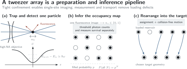
A tightly focused dipole trap supplies large curvature and optical access for single-particle fluorescence. Loading produces a stochastic binary occupancy map, so the probability of a fully occupied $N$-site array is only $p^N$ for independent filling $p$. Imaging identifies occupied reservoir sites, and controlled transport maps a selected subset into the desired target geometry.

Generating Tweezer Arrays

Several optical architectures can create multiple focuses.

Method	Main capability	Main calibration liabilities
Acousto-optic deflector	fast steering and multi-tone dynamic arrays	frequency-dependent efficiency, RF intermodulation, beat notes
Spatial light modulator	flexible two-dimensional phase holograms	finite refresh rate, phase retrieval, zero order, aberrations
Digital micromirror device	programmable binary amplitude patterns	optical efficiency, diffraction orders, pixelation
Microlens array	passive, parallel, stable focus array	fixed geometry, fabrication nonuniformity, limited rearrangement
Scanned single focus	time-averaged programmable potential	duty cycle, scan-induced micromotion, parametric heating

Hybrid systems often use one element for a static reservoir array and a second mobile tweezer for transport.

Coherent addition and beat notes

If two same-frequency fields overlap, their electric fields add:

$$I \propto \left| \mathbf E_1+\mathbf E_2 \right|^2.$$

Uncontrolled relative phase then creates static interference fringes. If the tweezers have frequency difference $\delta\omega$, the cross term beats at $\delta\omega$. A beat much faster than motional response may average out, while one near $\omega_i$ or $2\omega_i$ can drive sloshing or parametric heating.

Orthogonal polarization, frequency offsets, spatial separation, and careful RF-tone design can suppress crosstalk, but each choice can introduce vector light shifts or polarization-dependent trapping.

Uniformity

For fixed geometry,

$$\omega_{i,j} \propto \sqrt{U_j}.$$

Small site-to-site depth variations therefore produce

$$\frac{ \delta\omega_i }{ \omega_i } \simeq \frac12 \frac{ \delta U }{ U }.$$

The same $\delta U$ can create differential transition shifts, unequal Raman sidebands, position-dependent loading, and nonuniform gate detunings. Uniform camera brightness is not a sufficient proxy for uniform depth: fluorescence depends on cooling detuning and collection as well as occupancy.

Useful site-resolved calibrations include:

• AC Stark spectroscopy;
• parametric or sloshing frequencies;
• survival under a calibrated depth ramp;
• sideband spectra;
• beam-power measurements corrected for optical transfer;
• loading and imaging response maps.

Why Rearrangement Is Needed

Suppose each of $N$ target sites loads independently with probability $p$. The probability of a defect-free array without rearrangement is

$$P_{\mathrm{full}} = p^N.$$

Even good local filling becomes poor global filling as $N$ grows. For $p=0.55$ and $N=50$,

$$P_{\mathrm{full}} \simeq 1.0\times10^{-13}.$$

Rearrangement changes the question. Load $M>N$ reservoir sites, image them, and ask whether at least $N$ particles are available. Under the independent Bernoulli model,

$$P_{\mathrm{supply}} = \sum_{k=N}^{M} \binom{M}{k} p^k \left( 1-p \right)^{M-k}.$$

This can be close to unity even when $p^N$ is tiny. Rearrangement does not make stochastic loading deterministic; it converts excess spatial resources plus measurement and control into a high-probability target.

Assignment and path planning

After imaging, the controller must:

1. classify the occupancy of every reservoir and target site;
2. select which particles to keep;
3. assign loaded sites to target sites;
4. choose collision-free trajectories;
5. transport particles without spilling or excessive excitation;
6. re-image or otherwise verify the result.

A minimum-cost matching can reduce total distance, but distance is not the only cost. One may penalize crossings, weak traps, risky handoffs, long holds, or motion through occupied sites. Path planning and assignment should therefore be separated from the optical actuation model.

If every move survives independently with probability $s$ and $L$ moves are needed, the move-survival factor is

$$P_{\mathrm{move}} \simeq s^L.$$

This simple product is useful for budgeting but can fail when errors share a common cause such as laser-power drift or a bad spatial region.

Quantum Transport in a Moving Tweezer

Consider one harmonic axis with a moving center $x_c(t)$:

$$H(t) = \frac{ p^2 }{ 2m } + \frac12m\omega^2 \left[ x-x_c(t) \right]^2.$$

Assume the particle starts in the motional ground state and the trap begins and ends at rest. The coherent excitation relative to the final trap is

$$\alpha(T) = - \sqrt{ \frac{ m\omega }{ 2\hbar } } e^{-i\omega T} \int_0^T \dot x_c(t) e^{i\omega t} dt.$$

The added mean occupation is

$$\Delta\bar n = |\alpha(T)|^2.$$

Transport is excitation-free in this model when the velocity waveform has zero Fourier component at $\omega$. Slow smooth motion accomplishes this adiabatically, but carefully shaped faster trajectories can also cancel the resonant component. Merely specifying the average speed is insufficient.

Acceleration tilts the trap in its comoving frame. A finite-depth tweezer can spill the particle even when the harmonic excitation formula predicts a small $\Delta\bar n$. The maximum acceleration must therefore be compared with the full restoring-force curve, and handoffs between stationary and mobile traps must preserve both depth and phase-space overlap.

For a stored internal superposition, motion also accumulates a differential phase:

$$\phi_{ba} = \int_0^T \delta\omega_{ba} \left[ \mathbf r(t),t \right] dt.$$

Coherent transport requires reproducible phase or an echo/calibration protocol, not only particle survival.

Cooling and State Preparation

Loading and rearrangement generally leave motional excitation. Subsequent cooling can improve localization, suppress Doppler dephasing, reduce interaction fluctuations, and prepare resolved motional states.

Sideband cooling

In a resolved-sideband protocol, a coherent transition removes one motional quantum and optical pumping resets the internal state. A minimal cycle is

$$|g,n\rangle \longrightarrow |e,n-1\rangle \longrightarrow |g,n-1\rangle.$$

The cooling transition linewidth must be narrow enough to distinguish motional sidebands in the relevant effective model. The red-to-blue sideband-area ratio for a thermal harmonic mode is

$$\frac{ A_{\mathrm{red}} }{ A_{\mathrm{blue}} } = \frac{ \bar n }{ \bar n+1 },$$

provided the probe is weak, sidebands are resolved, matrix elements are treated consistently, and the distribution is thermal.

Three-dimensional cooling requires coupling to all principal axes. High-NA polarization structure and unfavorable Raman-beam geometry can leave a weakly cooled mode.

Internal-state preparation

Optical pumping, microwave or Raman pulses, and coherent clock transitions can prepare hyperfine, Zeeman, nuclear-spin, electronic, rotational, or vibrational states. The preparation error budget should include:

• residual population outside the computational manifold;
• position-dependent Rabi frequency and detuning;
• differential light shifts;
• motional sidebands and Doppler phase;
• Raman scattering from the tweezer;
• magnetic-field and polarization drift.

State-preparation fidelity and occupancy must be measured separately. An empty site cannot be silently counted as successful preparation of a dark state.

Rydberg and Neutral-Atom Control

Optical tweezer arrays provide flexible particle positions while Rydberg excitation supplies strong, switchable interactions. For a ground state $|g_i\rangle$, Rydberg state $|r_i\rangle$, and $n_i=|r_i\rangle\langle r_i|$, a common rotating-frame model is

$$\begin{aligned} H = & \sum_i \left[ \frac{ \hbar\Omega_i }{ 2 } \left( e^{i\phi_i} |r_i\rangle\langle g_i| + \mathrm{h.c.} \right) - \hbar\Delta_i n_i \right] \\ & + \sum_{i<j} V_{ij} n_in_j. \end{aligned}$$

For a van der Waals regime,

$$V_{ij} \simeq \frac{ C_6 }{ R_{ij}^6 }.$$

Blockade requires the interaction angular-frequency scale

$$B_{ij} = \frac{ |V_{ij}| }{ \hbar }$$

to exceed the excitation rate, detuning spread, linewidth, and relevant inhomogeneities. Finite blockade alone often contributes an error of order

$$\epsilon_{\mathrm{bl}} \sim \left( \frac{ \Omega }{ B } \right)^2,$$

with protocol-dependent coefficients.

The tweezer is not a passive spectator during a Rydberg pulse:

• ground and Rydberg states can have very different polarizabilities;
• the Rydberg state may be weakly trapped or anti-trapped;
• traps may be switched off, modulated, or tuned near a special condition;
• thermal motion creates Doppler detuning and optical phase noise;
• position fluctuations change $R_{ij}$ and therefore $V_{ij}$;
• loss can be confused with a logical state during readout.

Rydberg Atoms develops the excitation, trapping, detection, and calibrated-array stack; Rydberg Blockade develops collective dynamics, gates, and constrained models. Here the central lesson is operational: interaction fidelity depends on the entire loading–cooling–positioning–readout chain.

Molecules, Alkaline-Earth Atoms, and Clocks

Tweezers are not restricted to alkali atoms.

Molecules

Single molecules can be loaded by direct laser cooling or assembled from individually trapped atoms. Their additional rotational, vibrational, and hyperfine structure introduces anisotropic polarizability, dense Raman channels, and collision chemistry. A molecule can remain physically trapped while leaving the intended internal manifold, so state-resolved detection is essential.

Merging two tweezers permits controlled two-particle collisions or association. The relative motional ground state, species-dependent trap centers, differential sag, and state-dependent light shifts determine the short-range wave-function overlap.

Alkaline-earth-like atoms

Two-valence-electron atoms offer narrow intercombination and clock transitions alongside strong imaging transitions. This supports narrow-line cooling, nuclear-spin qubits, and magic trapping, but also requires careful control of metastable-state loss and state-dependent polarizability.

Metrology

Tweezer clocks combine single-particle readout with optical-clock spectroscopy. Their uncertainty budget includes site-resolved light shifts, collisional effects, motional sampling, dead time, atom-number fluctuations, and selection bias from postselection or rearrangement. Precision Spectroscopy owns the broader inference and systematic-error framework.

Worked Scale Audit

Consider an $^{87}\mathrm{Rb}$ atom in a red-detuned tweezer with assumed depth

$$\frac{ U_0 }{ k_{\mathrm B} } = 1.0\,\mathrm{mK},$$

measured $1/e^2$ waist

$$w_0 = 0.90\,\mu\mathrm m,$$

and wavelength

$$\lambda_L = 850\,\mathrm{nm}.$$

Using the paraxial Gaussian formulas as estimates, the Rayleigh range is

$$z_R = \frac{ \pi w_0^2 }{ \lambda_L } \simeq 2.99\,\mu\mathrm m.$$

For

$$m = 1.443\times10^{-25}\,\mathrm{kg},$$

the trap frequencies are

$$\frac{ \omega_r }{ 2\pi } \simeq 109\,\mathrm{kHz}, \qquad \frac{ \omega_z }{ 2\pi } \simeq 23.3\,\mathrm{kHz}.$$

The ground-state lengths are

$$x_{0,r} \simeq 23\,\mathrm{nm}, \qquad x_{0,z} \simeq 50\,\mathrm{nm}.$$

For a single 780 nm photon projected along a radial principal axis,

$$\eta_r \simeq \frac{ 2\pi }{ 780\,\mathrm{nm} } x_{0,r} \simeq 0.19.$$

A counterpropagating Raman pair can have nearly twice this wave-vector change, while a copropagating pair can have much less. The radial level spacing is

$$\frac{ \hbar\omega_r }{ k_{\mathrm B} } \simeq 5.25\,\mu\mathrm K.$$

Thus a temperature of $20\,\mu\mathrm K$ is cold in everyday units but not near the radial motional ground state without further cooling. The example also illustrates why a measured vector point-spread function and Hessian should replace the paraxial estimate in precision work.

Performance Ledger

A trustworthy array report keeps preparation, control, and readout metrics separate.

Layer	Primary metrics	Frequent hidden variable
trap	depth, $\omega_i$, lifetime, site spread	aberration and polarization
loading	$P(n=1)$, correlations, loading time	light-assisted collision branch
imaging	confusion matrix, survival, crosstalk	loss during exposure
rearrangement	supply probability, move count, success	correlated optical drift
motion	$\bar n_i$, heating, transport excitation	weak axial mode
internal state	preparation and gate fidelity	differential light shift
interaction	coupling distribution, decay, leakage	position and Doppler spread
final readout	state confusion plus loss detection	empty-site postselection

An end-to-end success probability is not obtained by quoting the best number from each layer. The layers are conditional and often correlated. For example, a deeper site may load better but scatter more, image brighter, shift a qubit farther, and transport differently.

Common Mistakes

“A tweezer is just a small Gaussian dipole trap”

The Gaussian model gives useful scales, but high-NA vector fields, aberrations, polarization gradients, and measured point-spread functions can control precision behavior.

“Fifty percent loading is fundamental”

The $1/2$ result follows from a two-in, zero-out collision model. Engineered collisions, alternative loading, and rearrangement can exceed it.

“High average filling means a defect-free array”

Without rearrangement, independent per-site filling $p$ gives global filling $p^N$, which falls exponentially with target size.

“A bright spot proves one particle is present”

Counts require a calibrated classifier. Two particles can collide during imaging, an occupied particle can be lost, and neighboring point-spread functions can create false counts.

“High detection fidelity means nondestructive readout”

Classification fidelity and survival are different conditional probabilities and must be reported separately.

“Slow transport is always necessary”

Slow motion is a robust route to low excitation, but shaped trajectories can cancel resonant Fourier components. Conversely, nominally slow motion can heat if it contains jitter near a trap frequency.

“Survival proves coherence”

A particle can remain trapped while accumulating an uncontrolled differential phase, changing internal state, or heating.

“Rydberg blockade is set only by spacing”

Blockade also depends on state, angle, excitation rate, detuning, linewidth, motion, and the distribution of actual interparticle distances.

Experimental Audit Checklist

1. Measure the optical focus. State the waist convention, effective NA, aberration correction, polarization, and objective-to-atom registration.
2. Calibrate each site’s potential. Measure depth, normal modes, differential shifts, and long-term drift.
3. Model loading transitions. Distinguish two-in, zero-out from two-in, one-out events and report site correlations.
4. Publish the imaging confusion matrix. Include background drift, neighboring-site crosstalk, and atom loss during exposure.
5. Report survival separately. Repeat imaging to infer nondestructive performance.
6. Validate the occupancy map. Correct rearrangement statistics for false positives and false negatives.
7. Budget rearrangement. Report supply probability, move count, path length, move survival, and added motional occupation.
8. Measure every motional axis. A cold radial mode can hide a hot weak axis.
9. Track internal-state purity and phase. Empty-site postselection must not masquerade as state fidelity.
10. Close the end-to-end loop. Verify the final target geometry and state after the complete experimental sequence.

References

1. R. Grimm, M. Weidemüller, and Y. B. Ovchinnikov, “Optical dipole traps for neutral atoms,” Advances in Atomic, Molecular, and Optical Physics 42, 95–170 (2000), doi:10.1016/S1049-250X(08)60186-X.
2. N. Schlosser, G. Reymond, I. Protsenko, and P. Grangier, “Sub-Poissonian loading of single atoms in a microscopic dipole trap,” Nature 411, 1024–1027 (2001), doi:10.1038/35082512.
3. N. Schlosser, G. Reymond, and P. Grangier, “Collisional blockade in microscopic optical dipole traps,” Physical Review Letters 89, 023005 (2002), doi:10.1103/PhysRevLett.89.023005.
4. T. Grünzweig, A. Hilliard, M. McGovern, and M. F. Andersen, “Near-deterministic preparation of a single atom in an optical microtrap,” Nature Physics 6, 951–954 (2010), doi:10.1038/nphys1778.
5. B. J. Lester, N. Luick, A. M. Kaufman, C. M. Reynolds, and C. A. Regal, “Rapid production of uniformly filled arrays of neutral atoms,” Physical Review Letters 115, 073003 (2015), doi:10.1103/PhysRevLett.115.073003.
6. Y. Miroshnychenko, W. Alt, I. Dotsenko, L. Förster, M. Khudaverdyan, D. Meschede, D. Schrader, and A. Rauschenbeutel, “An atom-sorting machine,” Nature 442, 151 (2006), doi:10.1038/442151a.
7. D. Barredo, S. de Léséleuc, V. Lienhard, T. Lahaye, and A. Browaeys, “An atom-by-atom assembler of defect-free arbitrary two-dimensional atomic arrays,” Science 354, 1021–1023 (2016), doi:10.1126/science.aah3778.
8. M. Endres, H. Bernien, A. Keesling, H. Levine, E. R. Anschuetz, A. Krajenbrink, C. Senko, V. Vuletić, M. Greiner, and M. D. Lukin, “Atom-by-atom assembly of defect-free one-dimensional cold atom arrays,” Science 354, 1024–1027 (2016), doi:10.1126/science.aah3752.
9. A. M. Kaufman, B. J. Lester, and C. A. Regal, “Cooling a single atom in an optical tweezer to its quantum ground state,” Physical Review X 2, 041014 (2012), doi:10.1103/PhysRevX.2.041014.
10. J. D. Thompson, T. G. Tiecke, A. S. Zibrov, V. Vuletić, and M. D. Lukin, “Coherence and Raman sideband cooling of a single atom in an optical tweezer,” Physical Review Letters 110, 133001 (2013), doi:10.1103/PhysRevLett.110.133001.
11. M. Saffman, T. G. Walker, and K. Mølmer, “Quantum information with Rydberg atoms,” Reviews of Modern Physics 82, 2313–2363 (2010), doi:10.1103/RevModPhys.82.2313.
12. A. Browaeys and T. Lahaye, “Many-body physics with individually controlled Rydberg atoms,” Nature Physics 16, 132–142 (2020), doi:10.1038/s41567-019-0733-z.
13. A. M. Kaufman and K.-K. Ni, “Quantum science with optical tweezer arrays of ultracold atoms and molecules,” Nature Physics 17, 1324–1333 (2021), doi:10.1038/s41567-021-01357-2.
14. A. Cooper, J. P. Covey, I. S. Madjarov, S. G. Porsev, M. S. Safronova, and M. Endres, “Alkaline-earth atoms in optical tweezers,” Physical Review X 8, 041055 (2018), doi:10.1103/PhysRevX.8.041055.
15. M. A. Norcia, A. W. Young, and A. M. Kaufman, “Microscopic control and detection of ultracold strontium in optical-tweezer arrays,” Physical Review X 8, 041054 (2018), doi:10.1103/PhysRevX.8.041054.
16. L. Anderegg, L. W. Cheuk, Y. Bao, S. Burchesky, W. Ketterle, K.-K. Ni, and J. M. Doyle, “An optical tweezer array of ultracold molecules,” Science 365, 1156–1158 (2019), doi:10.1126/science.aax1265.

Exercises

1. Tight-focus motional scales

For $^{87}\mathrm{Rb}$ with

$$m = 1.443\times10^{-25}\,\mathrm{kg},$$

take $U_0/k_{\mathrm B}=1.0\,\mathrm{mK}$, $w_0=0.90\,\mu\mathrm m$, and $\lambda_L=850\,\mathrm{nm}$. Estimate $z_R$, $\omega_r/(2\pi)$, $\omega_z/(2\pi)$, and $x_{0,r}$.

Solution

The Rayleigh range is

$$z_R = \frac{ \pi w_0^2 }{ \lambda_L } \simeq 2.99\,\mu\mathrm m.$$

Using $U_0=k_{\mathrm B}\times10^{-3}\,\mathrm K$,

$$\frac{ \omega_r }{ 2\pi } = \frac{1}{2\pi} \sqrt{ \frac{ 4U_0 }{ mw_0^2 } } \simeq 109\,\mathrm{kHz},$$

and

$$\frac{ \omega_z }{ 2\pi } = \frac{1}{2\pi} \sqrt{ \frac{ 2U_0 }{ mz_R^2 } } \simeq 23.3\,\mathrm{kHz}.$$

The radial ground-state length is

$$x_{0,r} = \sqrt{ \frac{ \hbar }{ 2m\omega_r } } \simeq 23\,\mathrm{nm}.$$

These are paraxial estimates; a high-NA field should be checked with the measured potential Hessian.

2. The collisional-blockade limit

Solve

$$\dot P_1 = R - \left( 2R+\gamma \right) P_1$$

for an initially empty site. Find the steady filling and loading time constant.

Solution

The linear equation has solution

$$P_1(t) = \frac{ R }{ 2R+\gamma } \left[ 1 - e^{-(2R+\gamma)t} \right].$$

Therefore

$$P_{1,\mathrm{ss}} = \frac{ R }{ 2R+\gamma }, \qquad \tau_{\mathrm{load}} = \frac{ 1 }{ 2R+\gamma }.$$

When $R\gg\gamma$, the steady filling approaches $1/2$.

3. One-particle-retaining collisions

Let a two-particle event leave one particle with probability $q=0.80$. Assume $R=20\,\mathrm{s^{-1}}$ and $\gamma=0.50\,\mathrm{s^{-1}}$. Find the steady single-particle filling.

Solution

The occupied-to-empty rate is

$$R(1-q)+\gamma = (20)(0.20)+0.50 = 4.50\,\mathrm{s^{-1}}.$$

Hence

$$P_{1,\mathrm{ss}} = \frac{ R }{ R+R(1-q)+\gamma } = \frac{ 20 }{ 24.5 } \simeq 0.816.$$

The improvement over $1/2$ comes from changing the collision branch, not from violating collisional blockade.

4. Supply probability for rearrangement

Twenty reservoir sites load independently with $p=0.60$. What is the probability that at least ten particles are available for a ten-site target? Compare this with the probability that ten fixed sites load without defects.

Solution

For rearrangement,

$$P_{\mathrm{supply}} = \sum_{k=10}^{20} \binom{20}{k} (0.60)^k (0.40)^{20-k} \simeq 0.872.$$

Without rearrangement, ten specified sites are all filled with probability

$$P_{\mathrm{fixed}} = (0.60)^{10} \simeq 6.05\times10^{-3}.$$

The reservoir converts extra sites into a much larger supply probability, but move and imaging errors still reduce the final success.

5. A photon-count threshold

Assume Poisson counts with $\mu_0=1$ for an empty site and $\mu_1=12$ for an occupied site. Classify the site as occupied for $n\ge5$. Calculate $P_{\mathrm{FP}}$, $P_{\mathrm{FN}}$, and the equal-prior classification fidelity.

Solution

The false-positive probability is

$$P_{\mathrm{FP}} = 1 - \sum_{n=0}^{4} e^{-1} \frac{ 1^n }{ n! } \simeq 3.66\times10^{-3}.$$

The false-negative probability is

$$P_{\mathrm{FN}} = \sum_{n=0}^{4} e^{-12} \frac{ 12^n }{ n! } \simeq 7.60\times10^{-3}.$$

Thus

$$F_{\mathrm{class}} = 1 - \frac{ P_{\mathrm{FP}}+P_{\mathrm{FN}} }{ 2 } \simeq 0.9944.$$

This number does not include particle loss during imaging and therefore is not an imaging-survival probability.

6. Excitation from a constant-velocity move

A harmonic tweezer moves by distance $d$ at constant velocity for time $T$, with instantaneous starts and stops:

$$\dot x_c(t) = \frac{d}{T}, \qquad 0<t<T.$$

Use the transport formula to find the added mean occupation.

Solution

The resonant Fourier integral is

$$\int_0^T \dot x_c(t) e^{i\omega t} dt = \frac{ d }{ T } \frac{ e^{i\omega T}-1 }{ i\omega }.$$

Its magnitude is

$$d \left| \frac{ \sin(\omega T/2) }{ \omega T/2 } \right|.$$

Therefore

$$\Delta\bar n = \frac{ m\omega d^2 }{ 2\hbar } \left[ \frac{ \sin(\omega T/2) }{ \omega T/2 } \right]^2.$$

The excitation vanishes in the ideal harmonic model when $\omega T=2\pi\ell$ for nonzero integer $\ell$. The instantaneous changes in velocity are experimentally unrealistic and can excite anharmonic modes, so smooth endpoint conditions are still desirable.

7. Depth uniformity from frequency data

Two nominally identical tweezer sites have radial frequencies that differ by $1.5\%$. Assuming their geometry is identical, estimate their fractional depth difference.

Solution

Because $\omega_r\propto\sqrt U$,

$$\frac{ \delta\omega_r }{ \omega_r } \simeq \frac12 \frac{ \delta U }{ U }.$$

Hence

$$\frac{ \delta U }{ U } \simeq 2 \left( 1.5\% \right) = 3.0\%.$$

This inference assumes equal waists and principal-axis geometry. A waist error can change frequency without the same proportional change in depth.

8. A blockade-scale audit

Two atoms have interaction energy $|V|/h=20\,\mathrm{MHz}$ and are driven with $\Omega/(2\pi)=2.0\,\mathrm{MHz}$. Estimate the finite-blockade error scale $(\Omega/B)^2$, where $B=|V|/\hbar$. Why is this not a complete gate error?

Solution

Since

$$B = \frac{ |V| }{ \hbar } = 2\pi \left( 20\,\mathrm{MHz} \right),$$

the ratio is

$$\frac{ \Omega }{ B } = \frac{ 2.0 }{ 20 } = 0.10.$$

Thus

$$\epsilon_{\mathrm{bl}} \sim 10^{-2}.$$

The coefficient depends on the pulse protocol, and the total error also includes Rydberg decay, laser phase and amplitude noise, Doppler detuning, position-dependent interaction, imperfect state preparation, leakage, trap switching, and readout error.