Rydberg Atoms Basics

A Rydberg atom has at least one electron in a state with large principal quantum number. That electron is weakly bound, far from the ionic core on atomic scales, and surrounded by a dense ladder of nearby levels. There is no universal integer at which an ordinary excited state becomes “Rydberg”; the useful criterion is a separation of scales between the extended electron and the compact core.

Rydberg states exaggerate atomic physics. Their orbital size, transition dipoles, electric polarizability, and interatomic interactions grow rapidly with effective principal quantum number, while binding energies and neighboring-level spacings shrink. The same amplification that makes them controllable also makes them sensitive to stray electric fields, blackbody radiation, motion, and nearby perturbing levels.

Canonical Scope

This page owns the atomic-physics bridge from high-$n$ structure to the first interaction and blockade models. Alkali Atoms owns the one-valence-electron core model and detailed quantum-defect conventions. Stark Effect in Atoms owns atom-specific static response and manifold mixing, while Dynamic Polarizability owns frequency-dependent response. The general perturbative origin of transition rates belongs to First-Order Transition Probability.

Optical Tweezers owns the loading, imaging, rearrangement, and motional preparation of site-resolved arrays. Rydberg Atoms builds from both pages to treat excitation, electric-field compensation, trapping, lifetime, readout, and array-level validation. Here the goal is to establish which scaling statements are controlled, why interactions become strong, and where the simple formulas fail.

Large Principal Quantum Number

For a hydrogenic electron outside a singly charged core, the binding energy relative to the series limit is approximately

$$E_n-E_{\mathrm{ion}} =- \frac{\mathcal R_M}{n^2},$$

where $\mathcal R_M$ is the isotope-appropriate Rydberg energy. The mean radius of a hydrogenic $|n\ell m\rangle$ state is

$$\langle r\rangle_{n\ell} = \frac{a_0}{2} \left[ 3n^2-\ell(\ell+1) \right].$$

At fixed low $\ell$, the radius grows as $n^2a_0$. A hydrogenic $50s$ state has $\langle r\rangle=3750a_0\simeq0.20\;\mu\mathrm m$, hundreds of nanometres rather than a fraction of a nanometre. Its binding energy is only about $5.4\;\mathrm{meV}$.

The adjacent-level spacing follows from differentiating the Coulomb energy:

$$|E_{n+1}-E_n| \sim \frac{2\mathcal R_M}{n^3}.$$

Thus an increasingly large atom has an increasingly dense spectrum. The Rydberg electron is far from the core much of the time, but low-$\ell$ wavefunctions can still penetrate it and acquire a substantial short-range phase shift.

Scaling Laws

For a nonhydrogenic one-valence-electron series, the natural variable is usually the effective principal quantum number

$$n^*=n-\delta_{\ell j},$$

not the printed integer $n$. The following asymptotic scalings are useful for fixed angular families away from accidental degeneracies:

Quantity	Typical scaling with $n^*$	Qualification
binding energy	$(n^*)^{-2}$	relative to one specified ionization threshold
adjacent-level spacing	$(n^*)^{-3}$	same series and large $n^*$
orbital radius	$(n^*)^2$	hydrogenic scale, with angular dependence
nearby-state electric-dipole matrix element	$(n^*)^2$	states connected by an allowed dipole channel
quadratic polarizability	approximately $(n^*)^7$	isolated low-$\ell$ states, away from degeneracies
spontaneous lifetime	approximately $(n^*)^3$	ordinary low-$\ell$ states at zero temperature
classical field-ionization scale	approximately $(n^*)^{-4}$	state- and ramp-dependent threshold
resonant dipole coefficient $C_3$	approximately $(n^*)^4$	angular factors and pair channel fixed
off-resonant van der Waals coefficient $C_6$	approximately $(n^*)^{11}$	away from Förster resonances

These are scaling estimates, not universal identities. Circular states have different lifetime behavior; blackbody-induced transitions alter room-temperature lifetimes; $C_6$ can change sign, cross zero, or become resonantly enhanced; and an electric field can reorganize the relevant basis before the nominal large polarizability can be used perturbatively.

Increasing $n$ is therefore not an unqualified improvement. Interactions grow, but level spacings shrink, field sensitivity increases, spectral crowding worsens, and the atom becomes easier to ionize.

Quantum Defects

An alkali-like Rydberg series converging to a chosen ionic level is described at leading order by

$$E_{n\ell j} = E_{\mathrm{ion}} - \frac{\mathcal R_M} {[n-\delta_{\ell j}(n)]^2}.$$

The quantum defect $\delta_{\ell j}$ summarizes the short-range phase accumulated through core penetration, exchange, polarization, relativistic structure, and channel mixing. It is tied to a specified series limit, isotope, and angular channel.

Low-$\ell$ electrons penetrate the core strongly and often have defects of order unity. A large centrifugal barrier keeps high-$\ell$ electrons outside the core, so their defects are usually small and their energies become nearly hydrogenic. This trend is qualitative: a defect may depend on energy and $j$, and a regular single-channel series can fail near a core excitation or configuration perturber.

The defect changes more than the binding energy. Replacing $n$ by $n^*$ gives a first organizing variable for radii, spacings, radial matrix elements, and lifetimes, but precision calculations still require actual wavefunctions and channel-resolved data. Central-Field Approximation explains the short-range effective potential, while the NIST term-series conventions in the references define how experimental series are reported.

Large Dipoles and Polarizability

A field-free atomic eigenstate of definite parity has no permanent electric dipole moment:

$$\langle n\ell jm| \mathbf d |n\ell jm\rangle =0.$$

Statements that “Rydberg atoms have huge dipoles” usually mean one of three more precise things:

1. Transition dipoles: nearby opposite-parity Rydberg states have radial matrix elements of order $ea_0(n^*)^2$.
2. Induced dipoles: weak fields admix nearby opposite-parity levels, producing a large quadratic response.
3. Stark-state dipoles: within a nearly degenerate hydrogenic manifold, a field-adapted superposition can have a permanent dipole of order $ea_0(n^*)^2$ along the field.

For an isolated nondegenerate level, the static polarizability is

$$\alpha_a(0) = 2\sum_{b\ne a} \frac{ |\langle b|d_z|a\rangle|^2 }{E_b-E_a}.$$

Combining $|d|\sim(n^*)^2$ with an energy denominator of order $(n^*)^{-3}$ gives the familiar estimate $\alpha\sim(n^*)^7$. Near degeneracy, however, nondegenerate second-order perturbation theory is the wrong tool: one must diagonalize the Stark Hamiltonian in the near-degenerate manifold.

This extreme response makes Rydberg levels excellent electrometers and tunable interaction states, but it also means that small patch fields and imperfect compensation can shift, mix, or ionize them.

Rydberg–Rydberg Interactions

At separations much larger than the electronic orbit, the leading electric dipole–dipole operator is

$$\begin{aligned} V_{dd}(\mathbf R) &= \frac{\mathcal A_{12}(\hat{\mathbf R})} {4\pi\varepsilon_0R^3},\\ \mathcal A_{12}(\hat{\mathbf R}) &= \mathbf d_1\cdot\mathbf d_2 \\ &\quad -3(\mathbf d_1\cdot\hat{\mathbf R}) (\mathbf d_2\cdot\hat{\mathbf R}). \end{aligned}$$

Even when each atom has zero diagonal dipole, $V_{dd}$ couples the prepared pair state $|rr\rangle$ to other pair states $|r'r''\rangle$. A minimal two-channel model is

$$H_{\mathrm{pair}} = \begin{pmatrix} 0 & V_{dd}\\ V_{dd}^* & \Delta_F \end{pmatrix},$$

where the Förster defect is

$$\Delta_F = E_{r'}+E_{r''}-2E_r.$$

Two limits follow.

Off-resonant pair coupling

If $|V_{dd}|\ll|\Delta_F|$, second-order perturbation theory gives

$$\Delta E_{rr} \simeq -\frac{|V_{dd}|^2}{\Delta_F} = \frac{C_6}{R^6}.$$

Because a nearby-state dipole scales approximately as $(n^*)^2$ and a typical pair-energy defect as $(n^*)^{-3}$, one obtains the rough estimate $C_6\sim(n^*)^{11}$. The sign depends on the energy denominator and channel composition.

Resonant pair coupling

When $|\Delta_F|\lesssim|V_{dd}|$, perturbative elimination fails. The pair states form an avoided crossing and the leading splitting scales as

$$\Delta E_{\pm} \sim \pm\frac{C_3}{R^3}.$$

Magnetic sublevels, quantization-axis orientation, electric and magnetic fields, and multiple nearby pair channels all matter. A scalar $C_6/R^6$ potential is therefore a model for a specified state and geometry, not a universal Rydberg force.

The multipole expansion also requires $R$ to exceed the electronic-cloud scale. At shorter range, overlap, exchange, molecular potentials, ionization, and higher multipoles invalidate the point-dipole picture.

Rydberg Blockade Preview

This section establishes the atomic-physics bridge and the conventional crossover scale. Rydberg Blockade owns the full bright-state reduction, finite-blockade phase and leakage, error-defined radii, collective superatoms, gate evidence, and projected many-body dynamics.

Consider two atoms with ground state $|g\rangle$, Rydberg state $|r\rangle$, single-atom Rabi frequency $\Omega$, and detuning $\Delta$. In the symmetric basis

$$|W_2\rangle = \frac{|gr\rangle+|rg\rangle}{\sqrt2},$$

the rotating-frame Hamiltonian can be written

$$H = \hbar \begin{pmatrix} 0 & \Omega/\sqrt2 & 0\\ \Omega/\sqrt2 & -\Delta & \Omega/\sqrt2\\ 0 & \Omega/\sqrt2 & -2\Delta+B \end{pmatrix},$$

where $B=V_{rr}/\hbar$ is the interaction shift in angular-frequency units. On resonance, $|B|\gg\Omega$ detunes $|rr\rangle$ and suppresses double excitation. The remaining transition $|gg\rangle\leftrightarrow|W_2\rangle$ has collective Rabi frequency $\sqrt2\,\Omega$.

For a van der Waals interaction, a commonly quoted blockade radius is defined by

$$\frac{|C_6|}{R_b^6} = \hbar\Omega_{\mathrm{eff}}, \qquad R_b = \left( \frac{|C_6|}{\hbar\Omega_{\mathrm{eff}}} \right)^{1/6}.$$

The comparison scale $\Omega_{\mathrm{eff}}$ may instead include linewidth, detuning, pulse bandwidth, or an error target. A blockade radius is therefore a convention-dependent crossover, not a hard boundary.

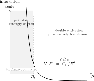
Schematic blockade criterion for $|V(R)|=|C_6|/R^6$. Inside $R_b$, the pair shift exceeds the chosen excitation scale $\hbar\Omega_{\mathrm{eff}}$; outside it, double excitation becomes progressively less detuned. The crossover is smooth and state dependent.

Finite blockade leaves a residual double-excitation amplitude, typically scaling as a power of $\Omega/B$ in an ideal pulse model. Spontaneous decay, Doppler shifts, laser phase noise, state leakage, inhomogeneous light shifts, and atomic motion produce additional errors.

From Two Atoms to Programmable Models

In an array, identify $|g_i\rangle$ and $|r_i\rangle$ with a two-level degree of freedom and define $n_i=|r_i\rangle\langle r_i|$. A widely used effective Hamiltonian is

$$\begin{aligned} H ={}& \frac{\hbar}{2} \sum_i\Omega_i\sigma_i^x -\hbar\sum_i\Delta_i n_i \\ &+\sum_{i<j}V_{ij}n_in_j. \end{aligned}$$

The laser drives local flips, detuning controls the excitation energy, and the geometry plus Rydberg pair potentials sets $V_{ij}$. In a strong nearest-neighbor blockade regime, configurations with adjacent Rydberg excitations are energetically suppressed. This creates constrained spin models and Ising-type Hamiltonians rather than a literal collection of independent two-level atoms.

Two broad uses follow:

• Analog quantum simulation: tune geometry, detuning, drive, and interaction range to study ordering, quenches, constrained dynamics, and nonequilibrium many-body phenomena.
• Quantum information processing: use blockade-dependent phases or collective excitation to mediate entangling operations between neutral-atom qubits.

The reduction is powerful but conditional. Leakage to other Rydberg levels, imperfect state preparation and readout, atom loss, finite temperature, and calibration errors remain physical parts of the platform. Demonstrating a programmable simulator or an entangling gate is not by itself evidence of fault-tolerant scalability.

Rydberg physics also supports electric-field sensing, microwave-to-optical transduction studies, nonlinear optics through interacting polaritons, and ultralong-range Rydberg molecules. Rydberg Electrometry develops the field-to-spectrum inverse problem, calibration chain, vapor-cell transfer, sensitivity, and bandwidth; the present page retains the underlying high-$n$ structure and scaling laws.

Practical Interpretation Checklist

Before applying a Rydberg scaling or pair potential, specify:

1. the species, isotope, ionic-core threshold, and effective quantum number $n^*$;
2. the complete electronic label, including $\ell$, $j$, magnetic sublevel, and parity;
3. electric and magnetic fields and the quantization-axis geometry;
4. the pair channel and Förster defect underlying $C_3$ or $C_6$;
5. whether the interatomic distance is large compared with the orbital radius;
6. the laser detuning, Rabi frequency, linewidth, and pulse bandwidth;
7. spontaneous, blackbody-induced, motional, and technical decoherence scales;
8. whether the desired result is a scaling estimate or a precision prediction.

Common Mistakes

• Using $n$ where a nonzero quantum defect requires $n^*$.
• Treating $(n^*)^7$ polarizability or $(n^*)^{11}$ interaction scaling as an exact law.
• Assigning a permanent dipole to a field-free parity eigenstate.
• Assuming $C_6$ is positive, isotropic, or independent of magnetic sublevel.
• Using $C_6/R^6$ through a Förster resonance where pair-state diagonalization is required.
• Calling $R_b$ a hard-sphere radius rather than a criterion-dependent crossover.
• Increasing $n$ without accounting for spectral crowding, field sensitivity, ionization, and blackbody transitions.
• Ignoring the finite size of the Rydberg orbit when atoms approach one another.
• Treating a driven many-body spin model as the complete atomic Hamiltonian.

Exercises

Exercise 1: Scaling from n = 25 to n = 50

For the same hydrogenic angular family, estimate how orbital radius, binding energy, adjacent-level spacing, quadratic polarizability, low-$\ell$ radiative lifetime, and off-resonant $C_6$ change when $n$ doubles from $25$ to $50$.

Solution

Using the asymptotic powers,

$$\begin{array}{ccl} \langle r\rangle\propto n^2 &\Longrightarrow& 4\ \text{times larger},\\ |E_b|\propto n^{-2} &\Longrightarrow& 1/4\ \text{as large},\\ \Delta E\propto n^{-3} &\Longrightarrow& 1/8\ \text{as large},\\ \alpha\propto n^7 &\Longrightarrow& 128\ \text{times larger},\\ \tau\propto n^3 &\Longrightarrow& 8\ \text{times longer},\\ C_6\propto n^{11} &\Longrightarrow& 2048\ \text{times larger}. \end{array}$$

The last three ratios are especially model dependent. They assume the same angular family, no nearby resonance, and no change in the dominant decay environment.

Exercise 2: Size and binding of a hydrogenic 50s state

Using $a_0=5.29\times10^{-11}\;\mathrm m$ and $\mathcal R_\infty=13.6\;\mathrm{eV}$, estimate the mean radius and binding energy of a hydrogenic $50s$ state.

Solution

For $\ell=0$,

$$\langle r\rangle = \frac32n^2a_0 =3750a_0.$$

Therefore

$$\begin{aligned} \langle r\rangle &\simeq 3750(5.29\times10^{-11}\;\mathrm m) \\ &=1.98\times10^{-7}\;\mathrm m \\ &=0.198\;\mu\mathrm m. \end{aligned}$$

The binding energy is

$$|E_b| = \frac{13.6\;\mathrm{eV}}{50^2} =5.44\times10^{-3}\;\mathrm{eV}.$$

This is a scale estimate for a hydrogenic state, not a precision alkali prediction.

Exercise 3: Two quantum defects

At $n=30$, compare a series with $\delta_s=3.10$ to one with $\delta_f=0.02$, assuming the same series limit and Rydberg energy. Which state is more deeply bound, and by what factor?

Solution

The effective quantum numbers are

$$n_s^*=26.90, \qquad n_f^*=29.98.$$

Because $|E_b|\propto1/(n^*)^2$,

$$\frac{|E_{b,s}|}{|E_{b,f}|} = \left( \frac{29.98}{26.90} \right)^2 \simeq1.24.$$

The core-penetrating $s$ state is about $24\%$ more deeply bound at the same printed $n$. The numerical defects are illustrative and do not define a real species without further data.

Exercise 4: Off-resonant pair shift

A pair channel has $C_3/h=2.0\;\mathrm{GHz}\,\mu\mathrm m^3$ and Förster defect $\Delta_F/h=200\;\mathrm{MHz}$. At $R=5.0\;\mu\mathrm m$, estimate the dipole coupling and the perturbative van der Waals shift in ordinary frequency units.

Solution

The dipole coupling is

$$\begin{aligned} \frac{V_{dd}}{h} &= \frac{C_3/h}{R^3} \\ &= \frac{2000\;\mathrm{MHz}\,\mu\mathrm m^3} {125\;\mu\mathrm m^3} \\ &=16\;\mathrm{MHz}. \end{aligned}$$

Its ratio to the defect is $16/200=0.08$, so second-order perturbation theory is plausible. The shift is

$$\frac{\Delta E_{rr}}{h} \simeq -\frac{(16\;\mathrm{MHz})^2} {200\;\mathrm{MHz}} =-1.28\;\mathrm{MHz}.$$

Angular factors and other pair channels have been absorbed into the illustrative $C_3$.

Exercise 5: Blockade radius

Suppose $|C_6|/h=1.0\;\mathrm{THz}\,\mu\mathrm m^6$ and the resonant single-atom Rabi frequency is $\Omega/(2\pi)=2.0\;\mathrm{MHz}$. Using $|C_6|/R_b^6=\hbar\Omega$, estimate $R_b$.

Solution

Dividing the criterion by $h$ gives

$$\frac{|C_6|/h}{R_b^6} = \frac{\Omega}{2\pi}.$$

Hence

$$\begin{aligned} R_b^6 &= \frac{10^{12}} {2.0\times10^6}\;\mu\mathrm m^6\\ &=5.0\times10^5\;\mu\mathrm m^6,\\ R_b &\simeq8.9\;\mu\mathrm m. \end{aligned}$$

Changing the bandwidth or acceptable double-excitation error changes the operational radius.

Exercise 6: Collective enhancement

For two noninteracting identical atoms driven resonantly with single-atom Rabi frequency $\Omega$, show that the drive couples $|gg\rangle$ to $|W_2\rangle=(|gr\rangle+|rg\rangle)/\sqrt2$ with collective Rabi frequency $\sqrt2\,\Omega$.

Solution

With

$$H_d = \frac{\hbar\Omega}{2} \sum_{i=1}^{2} \left( |r_i\rangle\langle g_i| +|g_i\rangle\langle r_i| \right),$$

acting on $|gg\rangle$ gives

$$H_d|gg\rangle = \frac{\hbar\Omega}{2} (|rg\rangle+|gr\rangle) = \frac{\hbar\Omega}{\sqrt2} |W_2\rangle.$$

A two-level Hamiltonian with Rabi frequency $\Omega_{\mathrm c}$ has off-diagonal element $\hbar\Omega_{\mathrm c}/2$. Therefore $\Omega_{\mathrm c}=\sqrt2\,\Omega$. Under blockade, the same enhancement survives while $|rr\rangle$ is shifted out of resonance.

Cross-Links

• Common Atomic Hamiltonians gives the pair-channel, van der Waals, resonant-dipole, and driven-array forms in one operator ledger.
• Atomic Physics
• Atomic Units and Scales
• Hydrogen as Atomic Prototype
• Central-Field Approximation
• Alkali Atoms
• Stark Effect in Atoms
• Atomic Selection Rules
• Rydberg Atoms Platform
• Rydberg Blockade
• Autler–Townes Splitting
• Electromagnetically Induced Transparency
• Rydberg Formula
• Dipole Transitions
• First-Order Transition Probability
• Adiabatic Elimination
• Lattice Models Overview
• AMO Physics Roadmap

References

1. T. F. Gallagher, Rydberg Atoms, Cambridge University Press, 1994, DOI: 10.1017/CBO9780511524530.
2. T. F. Gallagher, “Rydberg Atoms,” Reports on Progress in Physics 51, 143–188 (1988), DOI: 10.1088/0034-4885/51/2/001.
3. W. C. Martin and W. L. Wiese, “Term Series, Quantum Defects, and Spectral-Line Series,” in Atomic Spectroscopy: An Introduction, NIST, updated 2025, accessed 2026-07-21.
4. M. D. Lukin, M. Fleischhauer, R. Côté, et al., “Dipole Blockade and Quantum Information Processing in Mesoscopic Atomic Ensembles,” Physical Review Letters 87, 037901 (2001), DOI: 10.1103/PhysRevLett.87.037901.
5. D. Jaksch, J. I. Cirac, P. Zoller, et al., “Fast Quantum Gates for Neutral Atoms,” Physical Review Letters 85, 2208–2211 (2000), DOI: 10.1103/PhysRevLett.85.2208.
6. E. Urban, T. A. Johnson, T. Henage, et al., “Observation of Rydberg Blockade between Two Atoms,” Nature Physics 5, 110–114 (2009), DOI: 10.1038/nphys1178.
7. A. Gaëtan, Y. Miroshnychenko, T. Wilk, et al., “Observation of Collective Excitation of Two Individual Atoms in the Rydberg Blockade Regime,” Nature Physics 5, 115–118 (2009), DOI: 10.1038/nphys1183.
8. M. Saffman, T. G. Walker, and K. Mølmer, “Quantum Information with Rydberg Atoms,” Reviews of Modern Physics 82, 2313–2363 (2010), DOI: 10.1103/RevModPhys.82.2313.
9. I. I. Beterov, I. I. Ryabtsev, D. B. Tretyakov, and V. M. Entin, “Quasiclassical Calculations of Blackbody-Radiation-Induced Depopulation Rates and Effective Lifetimes of Rydberg $nS$, $nP$, and $nD$ Alkali-Metal Atoms,” Physical Review A 79, 052504 (2009), DOI: 10.1103/PhysRevA.79.052504.
10. H. Bernien, S. Schwartz, A. Keesling, et al., “Probing Many-Body Dynamics on a 51-Atom Quantum Simulator,” Nature 551, 579–584 (2017), DOI: 10.1038/nature24622.
11. A. Browaeys and T. Lahaye, “Many-Body Physics with Individually Controlled Rydberg Atoms,” Nature Physics 16, 132–142 (2020), DOI: 10.1038/s41567-019-0733-z.
12. S. Ebadi, T. T. Wang, H. Levine, et al., “Quantum Phases of Matter on a 256-Atom Programmable Quantum Simulator,” Nature 595, 227–232 (2021), DOI: 10.1038/s41586-021-03582-4.