Atomic Orbitals Revisited

An orbital is a normalized one-particle function, but that sentence does not yet say what role the function plays. In an exact one-electron atom it can be the complete spatial state. In a many-electron calculation it may instead be a basis function, a variational ingredient in a Slater determinant, an eigenfunction of an auxiliary operator, an eigenvector of a reduced density matrix, or a state-to-state removal amplitude.

Those objects are related, but they are not interchangeable. Much confusion about “seeing,” “occupying,” or assigning energy to an orbital comes from moving a statement valid in one context into another without carrying its assumptions.

The exact hydrogenic definition, $s,p,d,ldots$ notation, real and complex spherical-harmonic bases, and node counts are canonical in Atomic Orbitals. This page does not repeat that derivation. It develops the interpretation needed when orbitals are used for real atoms, molecules, correlated states, spectroscopy, and computation.

A Word with Several Precise Meanings

Context	Object called an orbital	Invariant physical content	Main caution
exact one-electron problem	eigenstate of the one-particle Hamiltonian	ray, density, currents, and matrix elements	phase and degenerate-basis choices remain conventional
finite-basis expansion	chosen one-particle basis function	the spanned subspace after convergence	a primitive basis function is not generally an eigenstate
Hartree–Fock	optimized spin-orbital in a single determinant	occupied projector and determinant	occupied canonical orbitals are not unique
Kohn–Sham theory	orbital of an auxiliary noninteracting system	density for the stated functional and solution	most eigenvalues are not exact removal energies
natural-orbital analysis	eigenfunction of the one-body density matrix	occupation spectrum and eigenspaces	degenerate occupations permit rotations
localized or hybrid analysis	unitary combination chosen for locality or interpretation	the retained orbital subspace	localization is method- and criterion-dependent
ionization or attachment	Dyson or quasiparticle amplitude	state-specific spectral amplitude	it is not a permanently occupied one-electron state

Whenever an article, plot, or program prints an “orbital,” first ask which row of this table applies.

Orbitals as One-Electron Wavefunctions

For one spinless particle, an orbital may be written as a ket $|\phi_p\rangle$ or a position-space wavefunction

$$\phi_p(\mathbf r)=\langle\mathbf r|\phi_p\rangle.$$

Including electron spin gives a spin-orbital

$$\chi_p(x)=\chi_p(\mathbf r,\sigma),$$

where $x$ abbreviates spatial and spin coordinates. In a collinear spin description it often factorizes as

$$\chi_p(x)=\phi_p(\mathbf r)\omega_p(\sigma),$$

with $\omega_p$ an $\alpha$ or $\beta$ spin function. Relativistic or noncollinear calculations use multicomponent spinors for which this product form need not hold.

Normalization means

$$\langle\chi_p|\chi_p\rangle =\sum_\sigma\int |\chi_p(\mathbf r,\sigma)|^2,d^3r=1.$$

An orthonormal set is convenient,

$$\langle\chi_p|\chi_q\rangle=\delta_{pq},$$

but nonorthogonal atomic and molecular basis functions are also legitimate. They require an overlap matrix and a generalized eigenvalue problem; orthogonality is not part of the dictionary definition of an orbital.

When the orbital is the whole state

For ideal hydrogen or a hydrogenic ion, the electron has no electronic partner with which to be entangled. A stationary orbital is then an exact eigenstate of the internal one-electron Hamiltonian, apart from the stated recoil, relativistic, radiative, and nuclear idealizations. Its energy is an eigenvalue of that Hamiltonian and its position probability density follows directly from the orbital.

This special case is conceptually clean but not generic. Once electron–electron interaction is present, the complete electronic state lives in an antisymmetric many-particle Hilbert space.

Orbitals Inside a Many-Electron State

For $N$ electrons, the coordinate wavefunction is

$$\Psi(x_1,x_2,\ldots,x_N),$$

antisymmetric under exchange of any two arguments. In general it cannot be assigned as a list in which “electron 1 occupies orbital $a$” and “electron 2 occupies orbital $b$.” The electron labels are argument slots, not persistent particle identities.

A chosen spin-orbital set generates Slater determinants $|\Phi_I\rangle$. A correlated state can be expanded as

$$|\Psi\rangle=\sum_I C_I|\Phi_I\rangle.$$

The coefficients and orbitals jointly represent the state. Changing the one-particle basis changes the determinant expansion, even when the many-electron vector represented by the full expansion does not change. The canonical construction of antisymmetric basis states belongs to Slater Determinants.

Occupation is controlled shorthand

Saying that a determinant “occupies orbitals $i,j,k$” means that those spin-orbitals define its occupied antisymmetric subspace. It does not attach a named electron to each function. In a superposition of determinants, even the occupation of a chosen orbital can be noninteger as an expectation value.

Occupation language remains useful when the reference determinant dominates or when an occupation-number basis has been explicitly chosen. It becomes misleading if it is promoted into a hidden classical assignment.

Electron Configurations develops the atomic subshell notation, Aufbau heuristic, core–valence partitions, and basis dependence of configuration weights built from these orbitals.

Probability Density and Nodes

For an exact one-electron spatial state,

$$\rho(\mathbf r)=|\phi(\mathbf r)|^2$$

is the position probability density. For a spin-orbital, sum over spin components. An isosurface drawn at $|\phi|^2=c$ or $|\phi|=c$ is a visualization choice, not a wall, trajectory, or boundary of the atom.

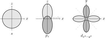
Common real-orbital sketches show selected isosurfaces and nodal geometry. The shaded signs encode relative wavefunction phase, not positive and negative charge. Atomic Orbitals owns the hydrogenic shapes and node counting; here the figure is reused to emphasize that an orbital rendering is a convention-dependent representation, not a directly photographed surface.

Density of a determinant

For a determinant of orthonormal occupied spin-orbitals, the spin-resolved one-particle density is a sum,

$$\rho(x)=\sum_{i\in\mathrm{occ}}|\chi_i(x)|^2.$$

The spatial electron density is obtained by summing over spin. Individual orbitals may have nodal planes while the total density remains nonzero there because other occupied orbitals contribute. It is therefore wrong to infer a node of the atom or molecule from a node in one chosen orbital.

Density of a correlated state

Write $X=(x_2,\ldots,x_N)$ and $dX=dx_2\cdots dx_N$. The one-body reduced density matrix is

$$\gamma(x,x') =N\int dX\, \Psi(x,X)\Psi^*(x',X).$$

Its diagonal gives the one-particle density,

$$\rho(x)=\gamma(x,x), \qquad \int \rho(x),dx=N.$$

This density is basis-independent. Decomposing it into orbital contributions is not unique unless an additional prescription, such as natural-orbital diagonalization, is stated.

Real and Complex Choices

Suppose a subspace $\mathcal S$ has orthonormal basis $\{|\phi_p\rangle\}$. Any unitary matrix $U$ defines another orthonormal basis,

$$|\widetilde\phi_a\rangle =\sum_p|\phi_p\rangle U_{pa}, \qquad U^\dagger U=I.$$

Real $p_x,p_y,p_z$ functions and complex $Y_1^m$ functions are familiar examples of different bases for the same angular-momentum subspace. Real orbitals display nodal planes conveniently; complex spherical harmonics diagonalize $L_z$.

Same subspace does not mean same individual state

A basis rotation preserves the subspace but generally changes each basis vector. If one electron is deliberately prepared in $p_x$ rather than $p_y$, those are different states and can produce different directional probabilities. The convention enters when no physical preparation, perturbation, or measurement distinguishes one basis within a degenerate subspace.

If two orbitals have different nondegenerate eigenvalues, their arbitrary linear combinations still span the same two-dimensional space but are not stationary eigenstates. “Any rotation is equivalent” is therefore a statement about a representation or occupied subspace, not a license to erase dynamics.

Phase can carry current

In the absence of a vector potential, a one-particle wavefunction has probability current

$$\mathbf j =\frac{\hbar}{m_e} \operatorname{Im}(\phi^*\nabla\phi).$$

A real stationary orbital has zero current under this formula, while a complex $L_z$ eigenstate can carry azimuthal current. Two basis choices can describe the same degenerate subspace, but selecting one complex state rather than a real superposition can change current-related observables. The canonical continuity-equation treatment is Probability Current.

Hybrid Orbitals as Basis Choices

Hybrid orbitals are linear combinations chosen to point along useful directions. Starting from orthonormal functions $s,p_x,p_y,p_z$, one tetrahedral convention is

$$\begin{aligned} 2h_1&=s+p_x+p_y+p_z,\\ 2h_2&=s+p_x-p_y-p_z,\\ 2h_3&=s-p_x+p_y-p_z,\\ 2h_4&=s-p_x-p_y+p_z. \end{aligned}$$

The four $h_i$ are orthonormal and span exactly the same four-dimensional space as the original $s$ and $p$ set. This is the mathematical content of idealized $sp^3$ hybridization.

What hybridization does and does not claim

In an isolated atom, $s$ and $p$ orbitals usually have different energies, so a hybrid is not a stationary eigenstate of the spherical atomic Hamiltonian. In a molecular environment, directional combinations may be useful for constructing a basis or interpreting a self-consistent occupied subspace.

Hybridization is therefore a representation adapted to geometry and bonding, not a literal time sequence in which an atom first promotes and mechanically mixes orbitals before a bond can form. Different localization schemes can produce different hybrids while preserving the same total wavefunction, density, or occupied projector. Valence Bond Theory shows how such directional bases enter localized, spin-coupled molecular structures.

Method-Dependent Orbitals

Hartree–Fock orbitals

Hartree–Fock optimizes a single Slater determinant. Its canonical spin-orbitals satisfy a self-consistent equation

$$f[P]|\phi_p\rangle =\epsilon_p|\phi_p\rangle,$$

where the Fock operator depends on the occupied projector $P$. For $N$ occupied spin-orbitals,

$$P=\sum_{i=1}^{N} |\phi_i\rangle\langle\phi_i|.$$

A unitary rotation among occupied orbitals leaves $P$ unchanged. The determinant changes only by the overall phase $\det U$, so its density and energy are unchanged. Canonical, localized, and symmetry-adapted occupied orbitals can therefore be different views of the same Hartree–Fock state.

Canonical virtual orbitals are even less intrinsic: they complete a convenient eigenbasis of the converged Fock operator but are not occupied particles. The full variational derivation, exchange operator, occupied-subspace invariance, and stability tests belong to Hartree–Fock Approximation; the radial, asymptotic, and open-shell atomic interpretation belongs to Hartree–Fock for Atoms.

Kohn–Sham orbitals

Kohn–Sham density-functional theory constructs an auxiliary noninteracting system whose ground-state density matches the interacting density for the exact functional. Its orbitals solve one-particle equations and are indispensable computational objects, but the auxiliary determinant is not generally the exact interacting wavefunction.

The exact highest occupied Kohn–Sham eigenvalue has a special relation to the ionization energy under the usual ground-state assumptions. This does not turn every occupied and virtual eigenvalue of an approximate functional into an exact photoelectron or excitation energy. Functional error, derivative discontinuities, symmetry breaking, and the chosen generalized Kohn–Sham framework matter.

Natural orbitals

Natural spin-orbitals diagonalize the one-body reduced density matrix:

$$\int \gamma(x,x')\varphi_k(x'),dx' =n_k\varphi_k(x).$$

The eigenvalues $n_k$ are natural occupation numbers. With a spin-orbital convention,

$$0\le n_k\le1, \qquad \sum_k n_k=N.$$

A single determinant has $N$ occupations equal to one and the rest zero. A correlated state generally has fractional occupations. In a spin-summed spatial-orbital convention, the upper bound is two instead; the convention must be stated.

Natural occupations are basis-independent eigenvalues of $\gamma$. Natural orbitals are unique up to phase only when their occupations are nondegenerate. Within a degenerate occupation subspace, unitary rotations remain allowed.

Localized orbitals

Localized orbitals are usually obtained by rotating an occupied or selected active subspace to optimize a criterion: spatial spread, atomic charge separation, bond localization, or another functional. Boys, Pipek–Mezey, intrinsic, and Wannier constructions do not generally produce the same orbitals.

Localization can make chemical structure and embedding approximations easier to interpret. It does not create a new many-electron state when the transformation is unitary within a complete occupied subspace. Report the localization criterion and the subspace to which it was applied.

Dyson orbitals

For ionization from an $N$-electron state $\Psi_N$ to a specified $(N-1)$-electron state $\Psi_{N-1}^{(a)}$, the Dyson orbital is the overlap amplitude

$$\begin{aligned} \mathcal I_a(x) &=\int dX\, \Psi_{N-1}^{(a)*}(X)\Psi_N(x,X),\\ \phi_D^{(a)}(x) &=\sqrt N\,\mathcal I_a(x). \end{aligned}$$

It connects two many-electron eigenstates and enters approximations to photoionization and electron-removal amplitudes. It need not coincide with a Hartree–Fock, Kohn–Sham, or natural orbital. Its norm measures state-specific one-electron character under the adopted normalization; correlation can distribute removal strength among many ionic channels.

Calling a reconstructed photoelectron amplitude “the orbital that the electron occupied” discards this state-to-state meaning.

Photoelectron Spectroscopy develops the measurement-level consequences: binding-energy conventions, Koopmans-style assignments, pole strengths, satellites, and continuum angular distributions.

Orbital Energies

An orbital does not carry an energy unless the method supplies an operator or convention that assigns one.

Orbital type	Meaning of a quoted energy
exact one-electron eigenstate	eigenvalue of the stated one-electron Hamiltonian
central-field model orbital	eigenvalue of the chosen effective potential; model-dependent
canonical Hartree–Fock orbital	eigenvalue of the Fock Lagrange-multiplier operator
Kohn–Sham orbital	eigenvalue of an auxiliary density-reproducing system
natural orbital	no intrinsic energy follows from diagonalizing $\gamma$
localized or hybrid orbital	any assigned energy requires an additional localization or block-partition convention
Dyson orbital	paired with a many-body removal energy, not its own eigenvalue in general

Koopmans’ frozen-orbital relation makes $-\epsilon_i^{\mathrm{HF}}$ an approximation to an ionization energy. Relaxation, correlation, state reorganization, and relativistic effects break a literal identification. Virtual Hartree–Fock energies are still less direct estimates of electron addition or neutral excitation.

The safe rule is simple: never quote an “orbital energy” without the generating operator, electron number, geometry, field conditions, and approximation.

What Is Observable?

An orbital function is usually not the eigenvalue of a universal Hermitian “orbital observable.” Experiments access quantities such as:

• total and transition energies;
• electron and spin densities;
• multipole moments and form factors;
• transition amplitudes, oscillator strengths, and lifetimes;
• momentum distributions and photoelectron angular distributions;
• scattering phases and ionization cross sections;
• response functions and spectral weights.

Orbitals help calculate and organize these observables. Inverse reconstruction can produce an orbital-like image only after choosing a forward model, gauge, phase convention, ionic channel, and treatment of experimental resolution. A successful reconstruction is evidence for that model-dependent amplitude, not a camera image of a classical electron path.

Density is not an orbital squared in general

For one electron, $\rho=|\phi|^2$. For a determinant, density is a sum over occupied orbitals. For a correlated state, it is the diagonal of $\gamma$. These three statements should not be collapsed into one slogan.

Likewise, a many-electron probability distribution contains pair and higher correlations that the one-body density cannot recover. Two states can share a similar density while differing in spin coupling, pair correlation, excitation spectrum, or entanglement.

Atomic and Chemical Language

Phrase	Controlled interpretation
atomic orbital	central-field eigenfunction or atom-centered one-particle basis function, depending on context
molecular orbital	one-particle function extended over a molecular electronic problem
basis function	primitive or contracted function used to expand orbitals; not necessarily an orbital eigenfunction
occupied orbital	member of the occupied subspace of a specified reference or noninteracting model
virtual orbital	unoccupied completion used by a specified method; representation-dependent
active orbital	member of a chosen subspace in which occupations or configurations are treated explicitly
bond or lone-pair orbital	localized representation selected by an analysis criterion
hybrid orbital	directional linear combination spanning a chosen atomic-like subspace

In atomic spectroscopy, symmetry labels such as $n\ell jm_j$ organize central-field and relativistic orbitals. In molecular calculations, point-group labels, localization, and bonding character often replace $\ell$ and $m$. In solids, Bloch and Wannier functions provide delocalized and localized bases for related band subspaces.

The vocabulary changes because the useful symmetry and approximation change. No single picture is privileged independently of the question.

Reading an Orbital Claim

Before trusting a statement about an orbital, identify:

1. System and Hamiltonian: one electron, fixed nuclei, relativistic level, external fields, and boundary conditions.
2. Method: exact eigenstate, model potential, Hartree–Fock, density functional, correlated wavefunction, or Green-function construction.
3. Coordinate and spin convention: spatial orbital, spin-orbital, two- or four-component spinor, real or complex basis.
4. Subspace: occupied, virtual, active, atomic, molecular, band, or ionic channel.
5. Transformation freedom: phases, degeneracies, occupied rotations, localization, and basis-set dependence.
6. Rendered quantity: amplitude, signed isosurface, density, difference density, current, or transition amplitude.
7. Observable connection: which measured quantity is predicted and how sensitive it is to the chosen representation.
8. Uncertainty and convergence: basis, grid, correlation, functional, relativistic, nuclear, and environmental errors.

An orbital picture with none of this metadata is an illustration, not a reproducible scientific result.

Common Mistakes

• Treating an orbital as a classical trajectory. A wavefunction is not a hidden path around the nucleus.
• Treating an isosurface as the edge of an atom. Its location changes when the plotting threshold changes.
• Reading lobe color as electric charge. It normally represents sign or phase; density is nonnegative.
• Assigning named electrons to orbitals. Identical-electron states are antisymmetric and do not preserve such identities.
• Assuming every orbital is unique. Phases, degeneracies, and unitary rotations within selected subspaces create legitimate alternatives.
• Assuming every basis rotation describes the same individual state. It preserves a subspace; a physically prepared vector can still differ.
• Equating one orbital’s nodes with nodes of the total density. Other orbitals or correlation can fill them.
• Calling hybridization a literal preparatory event. Hybrids are directional basis choices within a chosen subspace.
• Interpreting every orbital eigenvalue as a measured spectrum. The meaning depends on the generating operator and approximation.
• Calling a Dyson orbital an occupied mean-field orbital. It is an overlap between different electron-number states.
• Comparing orbital pictures from different methods without alignment. Phase, ordering, localization, geometry, and subspace must first be matched.

Exercises

1. Occupied-projector invariance

Let $\{|\phi_i\rangle\}_{i=1}^{N}$ be orthonormal occupied orbitals and define

$$|\widetilde\phi_a\rangle =\sum_{i=1}^{N}|\phi_i\rangle U_{ia},$$

where $U$ is unitary. Show that the occupied projector is unchanged.

Solution

The rotated projector is

$$\begin{aligned} \widetilde P &=\sum_a|\widetilde\phi_a\rangle \langle\widetilde\phi_a|\\ &=\sum_{aij}|\phi_i\rangle U_{ia}U_{ja}^*\langle\phi_j|. \end{aligned}$$

Unitarity gives

$$\sum_aU_{ia}U_{ja}^*=\delta_{ij},$$

so

$$\widetilde P =\sum_i|\phi_i\rangle\langle\phi_i|=P.$$

Any determinant built from the complete occupied set changes only by the phase $\det U$. Observables depending on the determinant or occupied projector are therefore unchanged, although plots of the individual rotated orbitals may look very different.

2. Orthonormal tetrahedral hybrids

Assume $s,p_x,p_y,p_z$ are orthonormal. Verify that the four $h_i$ defined in the hybrid-orbital section are normalized and mutually orthogonal. What has changed physically when this basis is adopted?

Solution

Each hybrid has four coefficients of magnitude $1/2$, so

$$\langle h_i|h_i\rangle =4\left(\frac12\right)^2=1.$$

For example,

$$\langle h_1|h_2\rangle =\frac14(1+1-1-1)=0.$$

Every other distinct pair has two matching and two opposite signs, so its inner product also vanishes. The coefficient matrix is a normalized Hadamard matrix and is unitary.

The one-particle subspace has not changed. Only its basis has been rotated. If a complete occupied or active-space treatment is transformed consistently, invariant observables are unchanged. The directional hybrids can still be more convenient for interpretation or approximation.

3. Natural occupations and idempotency

Use the spectral representation of the one-body density matrix to show that its natural occupations sum to $N$. Then explain why a single determinant has only occupations zero or one in a spin-orbital convention.

Solution

The spectral representation is

$$\gamma =\sum_k n_k|\varphi_k\rangle \langle\varphi_k|.$$

Taking the trace gives

$$\operatorname{Tr}\gamma =\sum_k n_k=N,$$

because the diagonal density integrates to the electron number.

For a determinant, $\gamma$ is the occupied projector $P$. Projectors are idempotent:

$$P^2=P.$$

Applying this equation to an eigenvector gives $n_k^2=n_k$, whose only real solutions are $n_k=0$ and $n_k=1$. Fractional natural occupations therefore diagnose departure from a single spin-orbital determinant, subject to the stated spin convention and numerical threshold.

4. Current in a complex angular state

Let

$$\phi(r,\theta,\varphi) =f(r,\theta)e^{im\varphi},$$

where $f$ is real. Derive its azimuthal probability current. Compare it with a real linear combination proportional to $f\cos(m\varphi)$.

Solution

Only the phase gradient contributes to the imaginary part:

$$\nabla(m\varphi) =\frac{m}{r\sin\theta}\,\mathbf e_\varphi.$$

Therefore

$$\mathbf j =\frac{\hbar m}{m_e r\sin\theta} |\phi|^2\mathbf e_\varphi.$$

The real function $f\cos(m\varphi)$ has zero probability current wherever the wavefunction is smooth because $\phi^*\nabla\phi$ is real. It is a superposition of opposite $m$ components rather than an $L_z$ eigenstate with eigenvalue $m\hbar$. The complex and real bases span the same $m,-m$ subspace, but preparing one particular vector can change current and angular-momentum observables.

5. Orbital nodes versus total density

Two orthonormal occupied spatial orbitals are rotated according to

$$\begin{aligned} \widetilde\phi_1 &=\cos\alpha\,\phi_1+sin\alpha\,\phi_2,\\ \widetilde\phi_2 &=-\sin\alpha\,\phi_1+cos\alpha\,\phi_2. \end{aligned}$$

Show pointwise that their summed density is invariant. What does this imply about interpreting a node in one localized or canonical orbital?

Solution

Expanding both squared magnitudes gives

$$\begin{aligned} |\widetilde\phi_1|^2 &=\cos^2\alpha|\phi_1|^2 +\sin^2\alpha|\phi_2|^2\\ &\quad+2\sin\alpha\cos\alpha \operatorname{Re}(\phi_1^*\phi_2),\\ |\widetilde\phi_2|^2 &=\sin^2\alpha|\phi_1|^2 +\cos^2\alpha|\phi_2|^2\\ &\quad-2\sin\alpha\cos\alpha \operatorname{Re}(\phi_1^*\phi_2). \end{aligned}$$

Adding cancels the cross terms and uses $\sin^2\alpha+\cos^2\alpha=1$:

$$|\widetilde\phi_1|^2+|\widetilde\phi_2|^2 =|\phi_1|^2+|\phi_2|^2.$$

Individual nodal surfaces can move under the rotation while the occupied-space density stays fixed. A node in one plotted orbital is therefore not automatically a node in the total electron density or a basis-independent boundary.

Cross-Links

• Atomic Orbitals is the canonical home for hydrogenic orbital notation, shapes, real and complex bases, and node counting.
• Change of Basis develops the representation-independent Hilbert-space principle used throughout this page.
• Valence Bond Theory applies localized orbital bases to spin-coupled covalent, ionic, and resonance structures.
• Central-Field Approximation explains how many-electron atoms generate effective atomic orbitals and residual interactions.
• Electron Configurations explains how chosen orbitals become subshell occupations, configuration-state functions, and mixed atomic levels.
• Periodic Table from Quantum Mechanics connects those orbital labels to block capacities, shell interleaving, and measured ionization trends.
• Hartree Method shows how one class of auxiliary atomic orbitals is generated by a self-consistent direct field.
• Hartree–Fock for Atoms adds the atomic exchange operator, spherical reductions, and orbital-energy caveats.
• Alkali Atoms shows where one-active-electron orbital labels work especially well and where core structure enters.
• Slater Determinants constructs antisymmetric states from spin-orbitals.
• Hartree–Fock Approximation owns the variational orbital equations, occupied rotations, orbital energies, and correlation boundary.
• Reduced Density Matrices supplies the general partial-trace language behind one-body densities.
• Spherical Harmonics develops the angular basis underlying atomic $s,p,d,\ldots$ labels.

References

1. A. Szabo and N. S. Ostlund, Modern Quantum Chemistry: Introduction to Advanced Electronic Structure Theory (Dover, 1996), Chapters 2–3.
2. T. Helgaker, P. Jørgensen, and J. Olsen, Molecular Electronic-Structure Theory (Wiley, 2000), Chapters 2, 10, and 11, doi:10.1002/9781119019572.
3. R. McWeeny, Methods of Molecular Quantum Mechanics, 2nd ed. (Academic Press, 1992), Chapters 3–6.
4. P.-O. Löwdin, “Quantum Theory of Many-Particle Systems. I. Physical Interpretations by Means of Density Matrices, Natural Spin-Orbitals, and Convergence Problems in the Method of Configurational Interaction,” Physical Review 97, 1474–1489 (1955), doi:10.1103/PhysRev.97.1474.
5. S. F. Boys, “Construction of Some Molecular Orbitals to Be Approximately Invariant for Changes from One Molecule to Another,” Reviews of Modern Physics 32, 296–299 (1960), doi:10.1103/RevModPhys.32.296.
6. J. Pipek and P. G. Mezey, “A Fast Intrinsic Localization Procedure Applicable for ab initio and Semiempirical Linear Combination of Atomic Orbital Wave Functions,” Journal of Chemical Physics 90, 4916–4926 (1989), doi:10.1063/1.456588.
7. W. Kohn and L. J. Sham, “Self-Consistent Equations Including Exchange and Correlation Effects,” Physical Review 140, A1133–A1138 (1965), doi:10.1103/PhysRev.140.A1133.
8. A. I. Krylov, “From Orbitals to Observables and Back,” Journal of Chemical Physics 153, 080901 (2020), doi:10.1063/5.0018597.
9. R. M. Martin, Electronic Structure: Basic Theory and Practical Methods (Cambridge University Press, 2004), Chapters 6–12, doi:10.1017/CBO9780511805769.
10. F. Jensen, Introduction to Computational Chemistry, 3rd ed. (Wiley, 2017), Chapters 5–9.