Hartree–Fock for Atoms

Atomic Hartree–Fock theory is the variationally optimal single-determinant description of an atom for a specified electronic Hamiltonian and one-electron representation. It retains exact fermionic antisymmetry within that trial family and replaces the coupled many-electron equation by self-consistent one-electron equations containing two qualitatively different fields:

f[\gamma] = h+V_{\mathrm{dir}}[\rho]-K[\gamma].

The direct Coulomb field $V_{\mathrm{dir}}$ is local and depends on the electron density $\rho(\mathbf r)$ . The exchange operator $K$ is nonlocal, spin selective, and depends on the occupied one-body density matrix $\gamma$ . Both are generated by the same Coulomb interaction. Exchange is not an additional force appended to the Hamiltonian.

For atoms, the general Hartree–Fock construction acquires extra structure. Rotational symmetry permits angular reduction, closed shells generate spherical densities, open shells require a declared averaging or term-specific prescription, and the Coulomb kernel can be organized into radial Slater integrals and angular coefficients. These choices determine what an “atomic Hartree–Fock orbital” or “Hartree–Fock energy” actually means.

Canonical Scope

This page is the canonical home for the atomic interpretation and specialization of Hartree–Fock theory:

atomic spin-orbitals and the Slater-determinant reference;
direct and nonlocal exchange fields in an atom;
self-interaction cancellation and the asymptotic field of an occupied orbital;
spherical closed shells and radial Hartree–Fock equations;
open-shell, average-of-configuration, and term-dependent choices;
restricted, restricted-open-shell, unrestricted, and generalized variants in atomic language;
radial grids, numerical orbitals, and finite orbital bases;
atomic total energies, orbital energies, and Koopmans-style ionization estimates;
validation criteria and the physical effects missing from a single determinant.

Hartree–Fock Approximation owns the full determinant variational derivation, occupied-projector formulation, Roothaan–Hall equations, uniform-electron-gas example, and general stability analysis. Slater Determinants owns determinant construction and normalization. Slater Determinants in Atoms owns the mapping among atomic determinants, configurations, projection sectors, and configuration-state functions. Exchange and Correlation owns the conceptual taxonomy of direct interaction, exchange, and correlation. Detailed integral engines, basis-set libraries, SCF accelerators, and production software workflows belong to Computational QM.

Atomic Hamiltonian and Determinant Ansatz

In the fixed-nucleus, nonrelativistic Coulomb model and atomic units,

\begin{aligned} H_{\mathrm C} ={}& \sum_{i=1}^{N}h(i) +\sum_{i<j}\frac{1}{r_{ij}},\\ h(i) ={}& -\frac12\nabla_i^2-\frac{Z}{r_i}. \end{aligned}

Here $Z$ is the nuclear charge, $N$ is the electron number, and $r_{ij}=|\mathbf r_i-\mathbf r_j|$ . Finite nuclear mass, relativistic interactions, radiative corrections, and nuclear structure are separate changes to the Hamiltonian; their omission should not be mislabeled electron correlation.

Write $x=(\mathbf r,\sigma)$ for combined spatial and spin coordinates. Hartree–Fock restricts the normalized $N$ -electron state to one determinant of orthonormal spin-orbitals:

\Phi(x_1,\ldots,x_N) = \frac{1}{\sqrt{N!}} \det[\chi_p(x_q)].

The determinant changes sign when any two electron coordinates are exchanged. Antisymmetry is therefore exact inside the trial space. The approximation is the much stronger statement that one occupied $N$ -dimensional one-particle subspace is enough to describe the state.

For the Coulomb Hamiltonian, the determinant expectation value is

\begin{aligned} E_{\mathrm{HF}} ={}& \sum_i h_{ii} +\frac12\sum_{i,j} \left(J_{ij}-K_{ij}\right),\\ h_{ii} ={}& \int \chi_i^*(x)h\chi_i(x)\,dx, \end{aligned}

with direct and exchange integrals. In the next two equations, $r_{12}=|\mathbf r-\mathbf r'|$ :

\begin{aligned} J_{ij} ={}& \iint \frac{dx\,dx'}{r_{12}}\, |\chi_i(x)|^2 |\chi_j(x')|^2. \end{aligned}

\begin{aligned} K_{ij} ={}& \iint \frac{dx\,dx'}{r_{12}}\, \chi_i^*(x)\chi_j(x)\\ &\times \chi_j^*(x')\chi_i(x'). \end{aligned}

Stationary variation under the orthonormality constraints gives

f\chi_i = \sum_j\lambda_{ji}\chi_j.

The Hermitian multiplier matrix $\lambda$ can be diagonalized by a unitary rotation among occupied orbitals. In that canonical orbital representation,

f\chi_i=\epsilon_i\chi_i.

The occupied subspace and determinant are invariant under that rotation. Canonical orbitals are a useful representation of the Hartree–Fock state, not separately unique electron states.

The Atomic Fock Operator

For any test spin-orbital $\psi(x)$ , the direct and exchange operators generated by occupied orbital $j$ act as

\begin{aligned} (J_j\psi)(x) ={}& \left[ \int \frac{|\chi_j(x')|^2} {|\mathbf r-\mathbf r'|} \,dx' \right]\psi(x),\\ (K_j\psi)(x) ={}& \chi_j(x) \int \frac{\chi_j^*(x')\psi(x')} {|\mathbf r-\mathbf r'|} \,dx'. \end{aligned}

Thus

f = h+\sum_{j\in\mathrm{occ}}(J_j-K_j).

$J_j$ multiplies the test orbital by an electrostatic potential and is therefore local in position. $K_j$ samples the test orbital at all positions $\mathbf r'$ before returning a value at $\mathbf r$ , so it is nonlocal. A single local screened potential cannot reproduce the complete Hartree–Fock exchange action on every orbital.

It is often clearer to collect occupied information into spin-resolved density matrices,

\begin{aligned} \gamma_\sigma(\mathbf r,\mathbf r') &= \sum_{j\in\mathrm{occ},\sigma} \phi_j(\mathbf r) \phi_j^*(\mathbf r'),\\ \rho(\mathbf r) &= \sum_\sigma \gamma_\sigma(\mathbf r,\mathbf r). \end{aligned}

For a spatial test function $\varphi_\sigma$ in spin channel $\sigma$ ,

\begin{aligned} (V_{\mathrm{dir}}\varphi_\sigma)(\mathbf r) ={}& \left[ \int \frac{\rho(\mathbf r')} {|\mathbf r-\mathbf r'|} \,d^3r' \right] \varphi_\sigma(\mathbf r),\\ (K_\sigma\varphi_\sigma)(\mathbf r) ={}& \int \frac{\gamma_\sigma(\mathbf r,\mathbf r') \varphi_\sigma(\mathbf r')} {|\mathbf r-\mathbf r'|} \,d^3r'. \end{aligned}

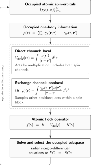
Atomic Hartree–Fock fixed-point structure showing local direct and nonlocal exchange channels — The same occupied orbitals generate a local direct potential through the diagonal density $\rho$ and a nonlocal, spin-resolved exchange operator through $\gamma_\sigma$ . Solving the resulting Fock equations supplies the next occupied subspace, so atomic Hartree–Fock is a nonlinear fixed-point problem.

Spin selection of exchange

If $\chi_i=\phi_i\alpha$ and $\chi_j=\phi_j\beta$ , then the spin overlap in $K_{ij}$ vanishes because $\langle\alpha|\beta\rangle=0$ . Direct Coulomb terms act between all occupied electrons, whereas exchange matrix elements survive only between spin-orbitals with overlapping spin components.

This does not make opposite-spin electrons distinguishable particles. Every determinant is antisymmetric under exchange of the complete spin-space coordinates. The vanishing matrix element follows from orthogonal spin functions within that representation.

Exact cancellation of one-orbital self-interaction

For $j=i$ ,

(J_i-K_i)\chi_i=0,

and equivalently $J_{ii}=K_{ii}$ . The direct field generated by an occupied spin-orbital does not act back on that same spin-orbital. Hartree–Fock therefore has no one-electron Coulomb self-interaction within its determinant energy.

This exact cancellation is orbital-channel specific. It does not imply that Hartree–Fock has the exact many-electron density, nor does it remove the interaction between distinct electrons.

Occupied-orbital asymptotic field

Far outside a finite atom, the nuclear and direct monopole terms behave as

-\frac{Z}{r}+\frac{N}{r}.

For an occupied orbital, its self-exchange monopole cancels one unit of the direct field. The diagonal occupied channel therefore has the Coulomb tail

V_i^{\mathrm{asymp}}(r) \sim -\frac{Z-N+1}{r}.

For a neutral atom, $Z=N$ , this is $-1/r$ . That tail is essential for the qualitative behavior of outer occupied orbitals. Because exchange is nonlocal, different occupied channels can also be asymptotically coupled; it is generally misleading to replace the result by one universal local “Hartree–Fock potential.”

An unoccupied canonical orbital is different: it has no occupied self-exchange term to cancel one unit of the direct field. In a neutral atom, the local nuclear-plus-direct monopole tends to zero, and the nonlocal exchange action on an orbital orthogonal to the occupied space is shorter ranged. Virtual Hartree–Fock orbitals therefore need not form the physical Rydberg or electron-attachment spectrum.

Spherical Atomic Reduction

For a nonrelativistic atom with a rotationally invariant reference, spin-orbitals can be chosen in the form

\chi_{n\ell m m_s}(x) = \frac{P_{n\ell}(r)}{r} Y_{\ell m}(\Omega) \eta_{m_s}(\sigma),

with radial normalization

\int_0^\infty P_{n\ell}(r)P_{n'\ell}(r)\,dr = \delta_{nn'}.

When every magnetic and spin state of a subshell is occupied, the subshell population is

q_{n\ell}=2(2\ell+1),

and its summed density is spherical. For closed shells,

\rho(r) = \frac{1}{4\pi r^2} \sum_{n\ell}q_{n\ell}P_{n\ell}^2(r).

Rotational invariance then permits orbitals with definite $\ell$ and $m$ , although the exchange operator remains nonlocal. Define the direct radial operator

\begin{aligned} \mathcal H_\ell^{\mathrm{dir}} ={}& -\frac12\frac{d^2}{dr^2} +\frac{\ell(\ell+1)}{2r^2}\\ &-\frac{Z}{r} +V_{\mathrm{dir}}(r). \end{aligned}

A schematic radial Hartree–Fock equation is then

\begin{aligned} \mathcal H_{\ell_a}^{\mathrm{dir}}P_a(r) &-\mathcal K_a[\{P_b\}](r)\\ &= \epsilon_aP_a(r). \end{aligned}

$\mathcal K_a$ denotes the angularly reduced exchange action. It is an integral operator involving occupied radial functions, not a multiplicative radial potential.

Coulomb multipoles and Slater integrals

The angular reduction starts from the multipole expansion

\begin{aligned} \frac{1}{|\mathbf r_1-\mathbf r_2|} ={}& \sum_{k=0}^{\infty} \frac{4\pi}{2k+1} \frac{r_<^k}{r_>^{k+1}}\\ &\times \sum_{q=-k}^{k} Y_{kq}^*(\Omega_1)Y_{kq}(\Omega_2), \end{aligned}

where $r_<=\min(r_1,r_2)$ and $r_>=\max(r_1,r_2)$ . Angular integration produces selection rules and numerical coefficients, while the radial dependence enters integrals of the form

\begin{aligned} R^k(ab,cd) ={}& \int_0^\infty\!dr_1\, P_a(r_1)P_c(r_1)\\ &\times \int_0^\infty\!dr_2\, \frac{r_<^k}{r_>^{k+1}}\\ &\times P_b(r_2)P_d(r_2). \end{aligned}

Direct Slater integrals are conventionally denoted $F^k$ and exchange integrals $G^k$ for suitable orbital assignments. Their radial values and their angular coefficients play different roles:

the radial integrals measure the strength of Coulomb overlap at each multipole rank;
angular coefficients determine which ranks contribute to a configuration or term;
the $k=0$ direct monopole supplies the spherical average;
higher multipoles and exchange distinguish terms built from the same occupation pattern.

Consequently, two atomic terms belonging to one electron configuration can have different Hartree–Fock energies even though their spherically averaged one-electron density is similar.

Closed-Shell Atomic Hartree–Fock

A closed-shell atom admits a spin-restricted reference in which each occupied spatial orbital is paired with $\alpha$ and $\beta$ spin. Every $m$ state of each occupied subshell is filled, so the density and Fock operator are rotational scalars.

The determinant is also an eigenstate with total spin $S=0$ and total orbital angular momentum $L=0$ . Neon, for example, has the nonrelativistic closed-shell reference

1s^2,2s^2,2p^6,

and each occupied $2p$ magnetic orbital shares the same radial function in a spherical restricted calculation.

Closed-shell symmetry is computationally useful, but it does not make the exact state a determinant. Opposite-spin electrons still avoid one another dynamically, and the exact wavefunction contains excited configurations even when its overall term is ${}^1S_0$ .

Helium as a special checkpoint

For a two-electron closed shell, the occupied spin-orbitals are $\phi\alpha$ and $\phi\beta$ . Acting on $\phi\alpha$ , the total direct field is $2J_\phi$ , while exchange with the occupied $\alpha$ orbital cancels one copy and exchange with $\beta$ vanishes. Hence

f\phi = (h+J_\phi)\phi = \epsilon\phi.

The total energy is

E_{\mathrm{RHF}} = 2h_{\phi\phi}+J_{\phi\phi}.

This spatial equation coincides with the optimized two-electron closed-shell Hartree equation. The equivalence is exceptional: it depends on two electrons sharing one spatial orbital with opposite spins. It does not mean exchange is absent, and it does not supply the missing explicit $r_{12}$ dependence. Helium Atom develops the resulting approximation ladder quantitatively.

Open-Shell Atoms

An open subshell does not fill every $m$ and spin state. A particular determinant may therefore select a spatial axis or spin projection even though the field-free Hamiltonian is rotationally invariant. It may have definite $M_L$ and $M_S$ without being an eigenstate of $L^2$ or $S^2$ .

Slater Determinants in Atoms shows how such projection-specific determinants are combined into symmetry-adapted CSFs before state-specific or multiconfiguration calculations.

There is no single universal object called “the open-shell atomic Hartree–Fock calculation.” One must state the variational and averaging prescription.

Average of configuration

Suppose a subshell $a=(n\ell)$ has degeneracy

g_a=2(2\ell+1)

and contains $q_a$ electrons. An equal-weight ensemble over all determinants in the configuration has a spherical one-body occupation

n_a=\frac{q_a}{g_a}

for every spin-orbital in the subshell. This average-of-configuration construction gives common radial orbitals and a rotationally averaged energy useful for organizing spectra and generating an orbital basis.

The two-particle average is not obtained by blindly multiplying fractional one-particle occupations. For two distinct spin-orbitals within the same subshell, the probability that both are occupied is

\frac{q_a(q_a-1)}{g_a(g_a-1)},

not $(q_a/g_a)^2$ . The distinction removes impossible self-pairs and gives the correct average of direct and exchange contributions over the fixed- $q_a$ configuration.

An average configuration is an ensemble or centroid construction. It is not a pure atomic term and should not be assigned a definite $L$ and $S$ merely because its radial density is spherical.

Term-dependent orbitals

For a specified symmetry $\alpha LS$ , an atomic energy can be organized schematically as

\begin{aligned} E(\alpha LS) ={}&E_{\mathrm{av}} +\sum_k a_k(\alpha LS)F^k\\ &+\sum_k b_k(\alpha LS)G^k. \end{aligned}

The angular coefficients $a_k$ and $b_k$ distinguish terms built from the same configuration. Optimizing orbitals for this energy gives a term-dependent self-consistent field. If the symmetry-adapted configuration-state function contains several determinants, the trial state is no longer literally one determinant even though the orbital equations retain Hartree–Fock-like direct and exchange structure.

This vocabulary matters when comparing tabulated atomic calculations. “Hartree–Fock,” “restricted Hartree–Fock,” “average level,” “average of configuration,” and “term-dependent Hartree–Fock” can refer to different stationary functionals and therefore different radial orbitals.

A lithium example

For the reference $1s^2,2s^1$ , a restricted-open-shell description pairs the two $1s$ electrons and leaves one $2s$ spin-orbital singly occupied. The outer electron feels the direct field of both core electrons but exchanges only with the same-spin core orbital. The closed-shell and open-shell radial equations consequently contain different combinations of direct and exchange terms.

No electron is permanently identifiable as “the outer electron.” The configuration labels an occupied subspace and coupling pattern; antisymmetry assigns no particle identity to an orbital.

Restricted and Unrestricted Variants

The adjective attached to Hartree–Fock specifies which orbital variations are allowed.

Variant	Orbital constraint	Atomic use	Main caution
restricted closed shell	paired $\alpha$ and $\beta$ electrons share each spatial orbital	closed-shell atoms and ions	cannot describe spin polarization
restricted open shell	closed-shell pairs share orbitals; open-shell orbitals obey a declared spin coupling	many high-spin open-shell references	canonical open-shell orbital energies are prescription dependent
unrestricted	$\alpha$ and $\beta$ electrons have independent spatial orbitals	spin-polarized atoms, ions, and broken-symmetry references	generally not an eigenstate of $S^2$
generalized	occupied spinors may mix $\alpha$ and $\beta$ components	noncollinear or spin-mixed references	interpretation and symmetry diagnosis are more involved
configuration averaged	open-shell magnetic substates are ensemble averaged	spherical atomic orbitals and configuration centroids	not a state-specific pure term

Unrestricted variation can lower the energy because it explores a larger determinant space. The lower value is not automatically a better approximation to a particular spectroscopic term: it may gain energy by breaking spin or spatial symmetry. A trustworthy comparison reports both the variational energy and symmetry diagnostics such as $\langle S^2\rangle$ .

Restricted-open-shell formulations also require care. The total stationary determinant may be well defined while different choices for canonicalizing closed, open, and virtual subspaces produce different orbital eigenvalues. Total energies and invariant subspaces are more fundamental than any one set of open-shell canonical orbital energies.

Atomic Self-Consistency

The Fock operator depends on the orbitals being solved for. In projector language, a stationary solution satisfies

[f[\gamma],\gamma]=0,

with $\gamma^2=\gamma$ for a pure determinant. An atomic self-consistent-field cycle is therefore:

Choose the electronic configuration, spin and spatial restrictions, Hamiltonian, and one-electron representation.
Build an initial occupied set from hydrogenic, screened, or previously converged orbitals.
Construct direct and exchange operators with the correct open-shell angular coefficients.
Solve the radial integro-differential equations or finite-basis matrix problem.
Select and orthonormalize the occupied subspace consistent with the target state.
Mix densities, projectors, or Fock matrices when needed and iterate to a fixed point.
Test equation residuals, energy stationarity, representation convergence, symmetry, and physical observables.

The SCF map can have several fixed points. A converged determinant may represent an excited occupancy, a saddle point, a broken-symmetry solution, or a higher local minimum. Repeating the calculation from physically distinct initial guesses is part of the method, especially for open shells and near-degenerate configurations.

Energy convergence is not enough

A small iteration-to-iteration energy change can coexist with a poor orbital residual. In a nonorthogonal finite basis, one useful residual is

R=FC-SC\varepsilon,

where $F$ is the Fock matrix and $S$ is the overlap matrix. In a radial representation, apply the final integro-differential operator to each orbital and inspect the norm of the residual directly.

A credible result checks at least:

changes in total energy and occupied projector;
orbital-equation residuals;
orthonormality and determinant idempotency;
radial-box, grid, or basis convergence;
near-origin and asymptotic behavior;
preservation or intentional breaking of angular and spin symmetries;
stability against occupied–virtual rotations when the ground-state minimum is claimed.

Radial Grids and Orbital Bases

Atomic symmetry permits representations that are less natural for general molecules. The representation is a numerical choice, not a change in Hartree–Fock theory.

Direct numerical radial orbitals

For a spherical atom, each $P_{n\ell}(r)$ can be represented on a finite-difference, finite-element, spline, spectral, or other radial grid. The calculation must resolve several disparate scales:

the near-nuclear region, where orbitals vary rapidly and behave as $P_{n\ell}(r)\propto r^{\ell+1}$ for a point nucleus;
shell and nodal structure at intermediate radii;
the diffuse tail of valence or weakly bound orbitals;
a sufficiently large outer boundary that does not distort the state.

Logarithmic or otherwise nonuniform grids are common because they place many points near the nucleus while retaining a large radial box. Coulomb multipoles can be evaluated through radial integral kernels or related Poisson equations. Exchange remains an orbital-dependent integral action.

Direct numerical methods are especially valuable for approaching the nonrelativistic radial Hartree–Fock limit without attributing finite orbital-basis error to the physical approximation.

Finite orbital bases

Alternatively, expand each spin-orbital in known functions,

\chi_i(x) = \sum_{\mu}C_{\mu i}\varphi_\mu(x).

Stationarity gives the generalized matrix equation

FC=SC\varepsilon.

Slater-type orbitals reproduce an exponential radial tail and can represent the nuclear cusp compactly. Gaussian-type orbitals make many-electron integrals especially efficient but have neither the exact point-nucleus cusp nor a pure exponential tail; systematic basis enlargement is therefore essential. Numerical atomic orbitals and $B$ -splines provide other useful compromises.

For any finite basis, report enough information to make the result reproducible: basis family, contraction or numerical construction, angular cutoff, treatment of diffuse and tight functions, nuclear model, and convergence thresholds.

Comparing representations

In nested variational orbital spaces, the minimized Hartree–Fock energy cannot rise as the space is enlarged. This monotonicity is a useful check, but it does not guarantee that every property converges monotonically. Radial discretization, quadrature, and boundary errors can also spoil simple variational ordering.

Agreement of total energies alone is insufficient. Hyperfine constants emphasize short distances, polarizabilities emphasize diffuse response, and transition amplitudes can be sensitive to cancellations. The representation must be converged for the observable being claimed.

Total Energies and Orbital Energies

For canonical occupied orbitals,

\epsilon_i = h_{ii} +\sum_j(J_{ij}-K_{ij}).

Summing over occupied orbitals counts every electron pair twice:

\sum_i\epsilon_i = \sum_i h_{ii} +\sum_{i,j}(J_{ij}-K_{ij}).

The total Hartree–Fock energy is therefore

\begin{aligned} E_{\mathrm{HF}} ={}& \sum_i\epsilon_i -\frac12\sum_{i,j} (J_{ij}-K_{ij}). \end{aligned}

Orbital eigenvalues are Lagrange multipliers associated with an optimized representation. The total electronic energy is not their sum, and differences of orbital energies are not generally exact atomic excitation energies.

Koopmans-style ionization

Remove occupied canonical spin-orbital $i$ while freezing all remaining $N-1$ orbitals. The determinant energy difference is

I_i^{\mathrm{frozen}} = E_{N-1}^{\mathrm{frozen}}(i)-E_N^{\mathrm{HF}} = -\epsilon_i.

This is Koopmans’ theorem in its original frozen-orbital form. It is an exact identity between two Hartree–Fock determinant energies under that constraint, not an exact theorem about the measured ionization spectrum.

If the ionic orbitals are reoptimized,

I_i^{\Delta\mathrm{SCF}} = E_{N-1}^{\mathrm{HF,opt}}(i) -E_N^{\mathrm{HF,opt}},

and relaxation lowers the optimized ionic energy relative to its frozen value. Correlation, relativistic shifts, spin-orbit splitting, finite nuclear mass, and the possibility of several ionic terms then further separate a measured threshold from $-\epsilon_i$ .

For inner shells, relaxation can be large. For open shells, removing one spin-orbital from a determinant can project onto several ionic terms, so one Koopmans number need not correspond to one spectral line.

Virtual eigenvalues require still more caution. They diagonalize the $N$ -electron Fock operator but do not include relaxation or correlation of the $(N+1)$ -electron ion and do not generally equal electron affinities. Neutral-atom virtual orbitals also lack the occupied-channel $-1/r$ self-exchange cancellation described above.

What Atomic Hartree–Fock Gets Right

Within the declared Hamiltonian and orbital space, Hartree–Fock provides:

a variational upper bound to the exact ground-state energy when the global determinant minimum is found;
exact antisymmetry and exact exchange for a single determinant;
cancellation of one-orbital Coulomb self-interaction;
a self-consistent shell and subshell structure;
useful zeroth-order orbitals for configuration interaction, many-body perturbation theory, coupled-cluster theory, and relativistic extensions;
often good qualitative densities and trends for compact closed-shell atoms;
a disciplined reference against which correlation energy can be defined.

Its success is strongest when one determinant dominates and the observable is not exceptionally sensitive to correlation or a missing Hamiltonian term.

What Hartree–Fock Misses

Correlation beyond one determinant

The exact Coulomb state can adjust its conditional motion beyond the exchange hole already enforced by antisymmetry. Conventional correlation energy is

E_{\mathrm{corr}} = E_0-E_{\mathrm{HF}} \le 0

for the same nonrelativistic Hamiltonian and one-electron space, with $E_{\mathrm{HF}}$ understood as the global determinant minimum. Comparing energies from different Hamiltonians or basis conventions does not isolate correlation.

Electron–electron cusp

The exact wavefunction has a specific short-range response as two electrons approach. A smooth one-electron orbital product cannot reproduce the full $r_{12}$ cusp, especially for opposite-spin pairs. This is one reason correlation expansions converge slowly in ordinary orbital bases.

Near-degenerate configurations

When several configurations have comparable amplitudes, selecting one determinant can give qualitatively wrong state ordering, dissociation behavior, or response. Beryllium’s mixing between $2s^2$ and $2p^2$ symmetry-adapted configurations is a standard atomic warning: a closed-shell determinant is useful, but the exact ${}^1S$ state is not structurally exhausted by it.

Relativity, recoil, and QED

Nonrelativistic Hartree–Fock does not contain spin-orbit interaction, the Breit interaction, finite nuclear mass, self-energy, vacuum polarization, or nuclear-size effects. These are Hamiltonian corrections, not correlation. For heavy atoms, a Dirac–Hartree–Fock or related relativistic starting point is often necessary before correlation is added.

Exact spectra and transition amplitudes

One determinant provides neither the full discrete spectrum nor exact photoionization, oscillator strengths, lifetimes, polarizabilities, or hyperfine properties. State-specific orbital relaxation and configuration mixing can be as important as the ground-state total energy suggests little about them.

Reading an Atomic Hartree–Fock Result

Before using a published or computed value, identify:

Hamiltonian: nonrelativistic Coulomb, Breit–Pauli, Dirac–Coulomb, finite-mass, or another model.
State prescription: closed-shell restricted, restricted open shell, unrestricted, configuration averaged, or term dependent.
Representation: direct radial grid, numerical orbitals, Slater functions, Gaussians, splines, or another basis.
Optimization target: total energy, configuration centroid, particular term, neutral atom, ion, or transition state.
Convergence evidence: residuals, basis or grid sequence, outer-boundary checks, and alternative SCF starts.
Observable layer: total energy, ionization difference, density, transition matrix element, or fitted spectroscopic parameter.
Missing physics: correlation, relativistic corrections, recoil, QED, nuclear size, external fields, or continuum coupling.

A result labeled simply “HF” is underspecified for precision work.

Common Mistakes

“Hartree–Fock neglects electron–electron repulsion”

It includes Coulomb repulsion through self-consistent direct and exchange terms. It neglects the residual correlation that requires a state more flexible than the chosen determinant reference.

“Exchange is a local correction to the Hartree potential”

Exact Hartree–Fock exchange is nonlocal. Local exchange potentials are different approximations or transformed descriptions and must be identified as such.

“Opposite-spin electrons do not need antisymmetrization”

The complete spin-space determinant is antisymmetric for every electron pair. Orthogonal spin functions merely make a particular exchange matrix element vanish.

“A spherical density proves the state has definite angular momentum”

An equal-weight configuration average is spherical but is generally an ensemble, not one pure $LS$ term. A broken-symmetry determinant can also yield useful radial averages without being an eigenstate of $L^2$ .

“The sum of orbital energies is the atomic energy”

The sum double counts every direct-minus-exchange pair contribution. The explicit half-pair correction is required.

“Minus the HOMO energy is the exact ionization energy”

$-\epsilon_{\mathrm{HOMO}}$ is a frozen-orbital Hartree–Fock removal energy. Orbital relaxation, correlation, multiplet structure, and other Hamiltonian corrections separate it from experiment.

“A lower unrestricted energy is automatically more accurate”

The larger variational space can lower the determinant energy by breaking a physical symmetry. Energy, spin contamination, angular symmetry, and the intended state must be assessed together.

“SCF convergence proves the ground state was found”

SCF equations have multiple stationary solutions. Residual convergence must be followed by stability tests, alternative starting guesses, and state identification.

“Every error relative to experiment is correlation energy”

Basis error, numerical error, finite nuclear mass, relativity, QED, nuclear size, and experimental conventions are separate contributions.

Exercises

Exercise 1: Self-interaction cancellation

For one occupied normalized spin-orbital $\chi_i$ , show directly that $(J_i-K_i)\chi_i=0$ .

Solution

The direct action is

(J_i\chi_i)(x) = \chi_i(x) \int \frac{|\chi_i(x')|^2} {|\mathbf r-\mathbf r'|} \,dx'.

The exchange action on the same orbital is

\begin{aligned} (K_i\chi_i)(x) ={}& \chi_i(x) \int \frac{\chi_i^*(x')\chi_i(x')} {|\mathbf r-\mathbf r'|} \,dx'\\ ={}&(J_i\chi_i)(x). \end{aligned}

Their difference vanishes pointwise. For a one-electron atom, the Hartree–Fock equation therefore reduces exactly to the one-electron Coulomb equation for the chosen Hamiltonian.

Exercise 2: The helium closed-shell equation

Take occupied spin-orbitals $\chi_1=\phi\alpha$ and $\chi_2=\phi\beta$ . Derive the Fock operator acting on $\phi\alpha$ and the total determinant energy.

Solution

The direct sum contains one contribution from each occupied spin-orbital:

J_1+J_2=2J_\phi.

Exchange with $\chi_1$ equals $J_\phi$ on $\phi\alpha$ , while exchange with $\chi_2$ vanishes because $\langle\alpha|\beta\rangle=0$ . Hence

f\phi = (h+2J_\phi-J_\phi)\phi = (h+J_\phi)\phi.

The one-body energy is $2h_{\phi\phi}$ . Of the pair terms, self terms cancel and the two ordered opposite-spin direct terms combine with the factor $1/2$ , giving

E_{\mathrm{RHF}} = 2h_{\phi\phi}+J_{\phi\phi}.

There is no opposite-spin exchange integral in this spin-orbital representation, but the full state is still an antisymmetric determinant.

Exercise 3: The outer occupied tail

An ion has nuclear charge $Z$ and $N$ occupied electrons. Use monopole counting to find the asymptotic Coulomb coefficient acting on an occupied Hartree–Fock orbital. Evaluate it for a neutral atom and for a singly positive ion.

Solution

At large $r$ , the nucleus contributes $-Z/r$ and the total direct density contributes $N/r$ . Self-exchange cancels one unit of direct charge in the occupied orbital’s own channel. Thus

V_i^{\mathrm{asymp}}(r) \sim -\frac{Z-N+1}{r}.

For a neutral atom, $N=Z$ , so the coefficient is $-1/r$ . For a singly positive ion, $Z-N=1$ , so it is $-2/r$ . Nonlocal exchange can couple occupied channels, so this monopole argument should not be reinterpreted as one exact local potential for every orbital.

Exercise 4: Fixed-configuration pair counting

A subshell contains $g$ spin-orbitals and exactly $q$ electrons, with every determinant in that configuration equally weighted. Find the occupation probability of one specified spin-orbital and the joint occupation probability of two distinct specified spin-orbitals. Compare the latter with the product of one-body probabilities.

Solution

There are $\binom{g}{q}$ determinants. A specified spin-orbital is occupied in $\binom{g-1}{q-1}$ of them, so

p_1 = \frac{\binom{g-1}{q-1}} {\binom{g}{q}} = \frac{q}{g}.

Two distinct specified spin-orbitals are jointly occupied in $\binom{g-2}{q-2}$ determinants, giving

p_2 = \frac{\binom{g-2}{q-2}} {\binom{g}{q}} = \frac{q(q-1)}{g(g-1)}.

In general,

p_2\ne p_1^2=\frac{q^2}{g^2}.

The fixed electron number induces combinatorial anticorrelation. Using $p_1^2$ in every pair term would count configurations that do not belong to the declared fixed- $q$ ensemble.

Exercise 5: Correct the orbital-energy sum

For an atomic determinant with occupied canonical orbitals, derive the total-energy correction to $\sum_i\epsilon_i$ . Then specialize to helium.

Solution

Summing the canonical equations gives

\sum_i\epsilon_i = \sum_i h_{ii} +\sum_{i,j}(J_{ij}-K_{ij}).

The determinant energy contains half the ordered pair sum, so

E_{\mathrm{HF}} = \sum_i\epsilon_i -\frac12\sum_{i,j}(J_{ij}-K_{ij}).

For helium, both occupied spin-orbitals have

\epsilon=h_{\phi\phi}+J_{\phi\phi}.

Therefore

E_{\mathrm{RHF}} = 2\epsilon-J_{\phi\phi} = 2h_{\phi\phi}+J_{\phi\phi}.

The direct interaction appears in each occupied eigenvalue and must be subtracted once from their sum.

Exercise 6: Frozen and relaxed ionization

Let $E_{N-1}^{\mathrm{frozen}}(i)$ be the energy after deleting occupied canonical orbital $i$ without changing the remaining orbitals, and let $E_{N-1}^{\mathrm{opt}}(i)$ be the minimum obtained by reoptimizing the ionic determinant within the same Hartree–Fock model. Establish the relation among the frozen, relaxed, and orbital ionization energies.

Solution

Koopmans’ frozen-orbital identity gives

E_{N-1}^{\mathrm{frozen}}(i)-E_N^{\mathrm{HF}} = -\epsilon_i.

The frozen ionic determinant is an allowed trial determinant for the optimized ion. Variational reoptimization therefore gives

E_{N-1}^{\mathrm{opt}}(i) \le E_{N-1}^{\mathrm{frozen}}(i).

Subtracting the same neutral energy yields

I_i^{\Delta\mathrm{SCF}} \le I_i^{\mathrm{frozen}} = -\epsilon_i

within the same Hamiltonian and orbital representation. This inequality isolates orbital relaxation inside Hartree–Fock. Correlation and other Hamiltonian corrections can shift the experimental ionization energy in either direction relative to these values.

Exercise 7: Diagnose an atomic calculation

A spherical unrestricted calculation for an open-shell atom has a lower energy than a restricted-open-shell calculation. Its energy and density changes are below threshold, but $\langle S^2\rangle$ differs substantially from the target $S(S+1)$ , the largest Fock residual is $10^{-4}$ hartree, and the valence orbital changes when the radial box is enlarged. What can and cannot be concluded?

Solution

The lower unrestricted energy follows from its larger variational space, but it does not establish a better approximation to the target spectroscopic term. The large error in $\langle S^2\rangle$ shows spin contamination or deliberate spin-symmetry breaking that must be interpreted. The Fock residual shows the reported orbitals are not yet stationary, and radial-box sensitivity shows the diffuse tail is unresolved.

No state-quality comparison is justified yet. The calculation should tighten the orbital solve, enlarge and refine the radial representation, repeat from several initial guesses, and compare energies only after both variants satisfy their own residual and representation-convergence criteria. The final report should include the symmetry diagnostics rather than quoting energy alone.

Key Takeaways

Atomic Hartree–Fock is a self-consistent direct-plus-exchange theory optimized within a declared determinant or closely related open-shell reference space.
The direct field is local and density generated; exact exchange is nonlocal and spin selective.
Same-orbital direct and exchange contributions cancel, giving occupied neutral-atom channels a $-1/r$ asymptotic Coulomb tail.
Closed shells permit a clean spherical restricted reduction, while open shells require a stated determinant, term-dependent, or configuration-average prescription.
Radial Slater integrals contain Coulomb strength; angular coefficients distinguish configurations and atomic terms.
Orbital energies are Lagrange multipliers. Their occupied sum double counts interactions, and Koopmans’ relation is a frozen-orbital ionization statement.
Radial grids and finite orbital bases solve the same Hartree–Fock problem but have different convergence errors.
A converged SCF fixed point is not necessarily the desired ground-state minimum or spectroscopic term.
Hartree–Fock contains exact determinant exchange but misses dynamical and multireference correlation, as well as physics absent from the chosen Hamiltonian.

Cross-Links

References

V. Fock, “Näherungsmethode zur Lösung des quantenmechanischen Mehrkörperproblems,” Zeitschrift für Physik 61, 126–148 (1930), doi:10.1007/BF01340294.
J. C. Slater, “Note on Hartree’s Method,” Physical Review 35, 210–211 (1930), doi:10.1103/PhysRev.35.210.2.
T. Koopmans, “Über die Zuordnung von Wellenfunktionen und Eigenwerten zu den Einzelnen Elektronen Eines Atoms,” Physica 1, 104–113 (1934), doi:10.1016/S0031-8914(34)90011-2.
D. R. Hartree, The Calculation of Atomic Structures, Wiley (1957).
C. Froese Fischer, The Hartree–Fock Method for Atoms: A Numerical Approach, Wiley (1977).
C. Froese Fischer, T. Brage, and P. Jönsson, Computational Atomic Structure: An MCHF Approach, Institute of Physics Publishing (1997).
R. D. Cowan, The Theory of Atomic Structure and Spectra, University of California Press (1981).
W. R. Johnson, Atomic Structure Theory: Lectures on Atomic Physics, Springer (2007).
I. P. Grant, Relativistic Quantum Theory of Atoms and Molecules: Theory and Computation, Springer (2007).
A. Szabo and N. S. Ostlund, Modern Quantum Chemistry: Introduction to Advanced Electronic Structure Theory, Dover (1996).
P.-O. Löwdin, “Correlation Problem in Many-Electron Quantum Mechanics. I. Review of Different Approaches and Discussion of Some Current Ideas,” Advances in Chemical Physics 2, 207–322 (1959), doi:10.1002/9780470143599.ch2.
E. Clementi and C. Roetti, “Roothaan–Hartree–Fock Atomic Wavefunctions,” Atomic Data and Nuclear Data Tables 14, 177–478 (1974), doi:10.1016/S0092-640X(74)80016-1.