Atomic Correlation Methods Overview

Atomic correlation methods enlarge, reorganize, or replace the single-determinant description of an interacting atom. They do not all approximate the same mathematical object in the same way. Configuration interaction expands a wavefunction linearly, many-body perturbation theory expands around a reference Hamiltonian, coupled cluster exponentiates connected excitations, density-functional theory makes the density primary, and quantum Monte Carlo estimates high-dimensional integrals or imaginary-time projections stochastically.

For a fixed nonrelativistic clamped-nucleus Hamiltonian, the conventional correlation energy is

$$E_{\mathrm c} = E_{\mathrm{exact}}^{\mathrm{NR,clamped}} -E_{\mathrm{HF}} \le 0.$$

The inequality follows because the Hartree–Fock determinant is a restricted variational trial state. This definition is precise only after the Hamiltonian, nuclear model, one-electron representation, symmetry sector, and Hartree–Fock reference have been fixed. It must not be confused with:

• the exchange-correlation functional of Kohn–Sham density-functional theory;
• the difference between a calculation and experiment;
• relativistic, recoil, finite-nuclear-size, or radiative corrections;
• the basis-set error in either the exact or Hartree–Fock calculation.

The practical question is therefore not “Which correlation method is best?” It is:

Which controlled approximation resolves the states and observables of this atom, for this Hamiltonian, to the required uncertainty?

Canonical Scope

This page is the canonical atomic method-selection map for:

• diagnosing single-reference, near-degenerate, and multireference atomic states;
• comparing configuration interaction, many-body perturbation theory, coupled cluster, density-functional theory, and continuum quantum Monte Carlo;
• understanding each method’s variational status, extensivity, dominant cost, and characteristic failure modes;
• choosing benchmark atoms and designing a convergence ladder;
• separating correlation-method uncertainty from basis, relativistic, recoil, QED, and data uncertainties.

It does not reproduce full generic derivations. Variational Many-Body States owns the general variational hierarchy, Perturbation Theory in Many-Body Systems owns linked expansions and denominator pathologies, and Quantum Monte Carlo Preview owns the general sampling and uncertainty pipeline. Hartree–Fock for Atoms owns the atomic reference problem. Electronic Structure Overview owns the molecular counterpart, including basis-set design, CASSCF, excited-state routes, and H₂ dissociation. The present page connects the atomic tools to structure and spectroscopy.

Why Correlation Matters

The exact nonrelativistic electronic Hamiltonian in atomic units is

$$\begin{aligned} H ={}& \sum_{i=1}^{N} \left( -\frac12\nabla_i^2-\frac{Z}{r_i} \right)\\ &+ \sum_{i<j}\frac{1}{r_{ij}}. \end{aligned}$$

Hartree–Fock optimizes the best single determinant for this Hamiltonian. It includes direct Coulomb effects and exact exchange within that determinant, but its pair density has the restricted form implied by independent occupied spin-orbitals. The exact wavefunction can correlate electron positions, spins, and configurations beyond that form.

The correlation hole

For a normalized state, the spin-summed pair density may be written

$$n_2(\mathbf r,\mathbf r') = n(\mathbf r) \left[ n(\mathbf r') +n_{\mathrm{xc}}(\mathbf r,\mathbf r') \right].$$

Here $n_{\mathrm{xc}}$ is an exchange-correlation hole conditional on an electron at $\mathbf r$. Its exchange part already appears for a determinant; its remaining correlation part describes additional rearrangement caused by the interaction. The hole obeys a particle-conservation sum rule under the usual normalization,

$$\int n_{\mathrm{xc}}(\mathbf r,\mathbf r') \,d^3r' =-1.$$

The detailed spatial shape matters. Short-range avoidance lowers Coulomb repulsion, but correlation can also move probability into other regions so that normalization and symmetry are preserved.

Cusp physics is not orbital relaxation

When two electrons approach one another, the Coulomb singularity imposes a cusp condition on the exact coordinate-space wavefunction. In atomic units, for the spherical average of an opposite-spin pair,

$$\left. \frac{\partial\overline\Psi}{\partial r_{12}} \right|_{r_{12}=0} = \frac12 \overline\Psi(0).$$

A finite expansion in smooth one-electron orbitals reproduces this nonanalytic dependence only slowly. Explicitly correlated coordinates, large orbital spaces, or Jastrow factors can represent it more efficiently. By contrast, allowing Hartree–Fock orbitals to relax changes the best determinant but does not create an explicit interelectronic coordinate.

Energies are unusually forgiving

The variational energy is stationary at an exact normalized eigenstate. If a normalized trial state differs by a small orthogonal component,

$$\lvert\widetilde\Psi\rangle = \sqrt{1-\epsilon^2}\, \lvert\Psi_0\rangle +\epsilon\lvert\Psi_\perp\rangle,$$

then its energy error begins at order $\epsilon^2$:

$$\widetilde E-E_0 = \epsilon^2 \left( \langle\Psi_\perp|H|\Psi_\perp\rangle-E_0 \right).$$

Many other observables have first-order wavefunction error. A method can therefore predict an excellent total energy while giving a visibly poorer contact density, hyperfine constant, polarizability, weak-interaction matrix element, or transition amplitude. Correlation quality is observable dependent.

Establish the Error Budget First

Before choosing a method, declare the target quantity and separate at least six error classes:

$$\begin{aligned} \Delta O ={}& \Delta O_{\mathrm{Hamiltonian}} +\Delta O_{\mathrm{basis}} +\Delta O_{\mathrm{corr}}\\ &+\Delta O_{\mathrm{rel/recoil/QED}} +\Delta O_{\mathrm{num}} +\Delta O_{\mathrm{data}}. \end{aligned}$$

The symbols are bookkeeping categories, not automatically independent random variables. Their uncertainties may be correlated. Still, the ledger prevents a common mistake: increasing the correlation rank while a radial box, one-particle basis, omitted relativistic term, or unresolved experimental assignment dominates the comparison.

Fix the physical target

A reproducible atomic calculation states:

• isotope and nuclear charge distribution;
• charge state and electron number;
• target parity, total angular momentum, and any nonrelativistic $L$ and $S$ labels;
• nonrelativistic, scalar-relativistic, Breit, recoil, and QED terms retained;
• whether energies are absolute, excitation, ionization, or affinity differences;
• the observable operator and whether it is transformed consistently with the wavefunction method;
• the basis, radial grid, box, continuum representation, and convergence thresholds.

Spectroscopic comparisons are energy differences between separately correlated states. Cancellation can help, but it is not guaranteed when the two states have different orbital relaxation or correlation structure.

Diagnose the Reference State

The first method choice is usually a state diagnosis, not a software choice.

Dynamic correlation

Dynamic correlation describes many individually small excitations that refine short-range avoidance and screening around a qualitatively correct reference. Closed-shell neon is a standard example: one determinant provides a useful zeroth-order state, but a large excitation space is needed for quantitative energy and response properties.

Static and near-degeneracy correlation

Static correlation arises when two or more configurations have comparable zeroth-order weights. It is common in open shells, stretched bonds, accidental degeneracies, and atoms such as beryllium where $2s^2$ and $2p^2$ configurations can mix importantly. A single determinant may then be qualitatively wrong even before fine dynamic correlation is added.

For a one-body reduced density matrix,

$$\gamma(\mathbf x,\mathbf x') = N \int \Psi(\mathbf x,\mathbf x_2,\ldots) \Psi^*(\mathbf x',\mathbf x_2,\ldots) \,d\mathbf x_2\cdots d\mathbf x_N,$$

natural spin-orbitals satisfy

$$\int \gamma(\mathbf x,\mathbf x') \varphi_p(\mathbf x') \,d\mathbf x' =n_p\varphi_p(\mathbf x).$$

For a single determinant, $n_p$ is exactly $1$ or $0$ in spin-orbital normalization. Several substantially fractional occupations indicate that one determinant is insufficient. They do not, by themselves, prescribe a unique method or threshold.

No universal diagnostic number

Large CI coefficients, natural occupations, coupled-cluster amplitudes, orbital-energy gaps, energy variance, and sensitivity to reference choice can all be informative. None is a universal pass/fail statistic across elements, basis sets, Hamiltonians, and observables. A defensible diagnosis combines several indicators with a physically chosen active space and state tracking.

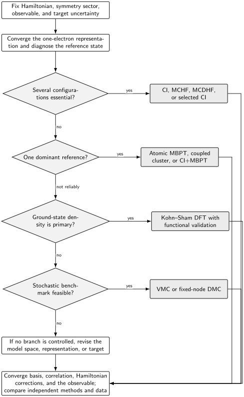
A method map, not a ranking. The branches identify useful starting points; every path returns to basis, correlation, Hamiltonian, and observable-specific validation. Hybrid strategies such as CI plus MBPT or multireference coupled cluster deliberately cross branches.

Configuration Interaction

Configuration interaction, or CI, expands the state in antisymmetric basis functions,

$$\lvert\Psi_K\rangle = \sum_I c_I^{(K)} \lvert\Phi_I\rangle.$$

The basis states may be Slater determinants or spin- and angular-momentum-adapted configuration state functions. Projecting the Schrödinger equation gives the matrix problem

$$\sum_J H_{IJ}c_J^{(K)} = E_Kc_I^{(K)}, \qquad H_{IJ} = \langle\Phi_I|H|\Phi_J\rangle.$$

Within a fixed finite one-electron basis and symmetry sector, diagonalizing the Hamiltonian in all allowed determinants gives full CI. Full CI is exact only for that finite representation. It still carries basis, box, nuclear-model, and Hamiltonian errors.

Variational ordering

If nested CI spaces satisfy

$$\mathcal V_1 \subset \mathcal V_2,$$

then their lowest Ritz energies obey

$$E_0(\mathcal V_2) \le E_0(\mathcal V_1).$$

This monotonicity is valuable, but only for the lowest state of the same symmetry in genuinely nested spaces. Excited roots can change character or exchange order; state tracking must use overlaps, dominant configurations, angular labels, and observables rather than root number alone.

Excitation-rank truncation

Starting from a determinant $\Phi_0$, a conventional hierarchy is

$$\lvert\Psi_{\mathrm{CISD}}\rangle = c_0\lvert\Phi_0\rangle +\sum_{ia}c_i^a\lvert\Phi_i^a\rangle +\frac14 \sum_{ijab}c_{ij}^{ab} \lvert\Phi_{ij}^{ab}\rangle.$$

Occupied labels are $i,j$ and virtual labels are $a,b$. Singles describe orbital relaxation and polarization in a fixed orbital basis; doubles are the lowest rank that directly describes pair correlation for a two-body Hamiltonian. Higher ranks become important through coupling and in multireference states.

Truncated CI is variational in its selected space but is not generally size extensive. For two noninteracting fragments $A$ and $B$, CISD omits products in which each fragment is simultaneously doubly excited, because that product is a quadruple excitation relative to the combined reference. Consequently,

$$E_{AB}^{\mathrm{CISD}} \ne E_A^{\mathrm{CISD}} +E_B^{\mathrm{CISD}}$$

even at infinite separation. This defect matters most for changing system size and dissociation, but it also warns against treating a truncated-CI energy as a uniformly balanced correlation measure.

Atomic CI is symmetry organized

Atomic calculations exploit exact labels such as parity $\pi$ and total angular momentum $J$ in a relativistic formulation, or $L$, $S$, $J$, and parity where an $LS$ description is appropriate. Instead of diagonalizing every determinant together, one constructs blocks such as

$$H^{J\pi}_{IJ} = \langle\Phi_I^{J\pi}|H|\Phi_J^{J\pi}\rangle.$$

This reduces cost and prevents forbidden mixing. It does not make configuration labels exact: different configurations with the same exact symmetry may mix strongly.

Multiconfiguration optimization

CI optimizes coefficients for fixed orbitals. Multiconfiguration Hartree–Fock and multiconfiguration Dirac–Hartree–Fock optimize both coefficients and orbitals,

$$\delta \frac{ \langle\Psi(\mathbf c,\boldsymbol\phi)|H|\Psi(\mathbf c,\boldsymbol\phi)\rangle }{ \langle\Psi(\mathbf c,\boldsymbol\phi)|\Psi(\mathbf c,\boldsymbol\phi)\rangle } =0.$$

An active-space sequence can then add layers of virtual orbitals and selected substitutions. The result is powerful for open-shell spectra and transition properties, provided the configuration-generation rule, orbital optimization strategy, and omitted classes are reported.

Selected CI and extrapolation

Selected CI retains determinants judged important by a perturbative estimate, variational criterion, or adaptive search. It can approach full CI in spaces too large for exhaustive enumeration. Selection thresholds introduce a new convergence coordinate, and extrapolation to zero threshold is method dependent. A small discarded perturbative correction is evidence only when the selection and basis sequences are stable.

Many-Body Perturbation Theory

Atomic many-body perturbation theory, or MBPT, partitions the Hamiltonian as

$$H = H_0+\lambda V,$$

and expands an energy, wave operator, matrix element, or effective Hamiltonian in $\lambda$. A common choice makes $H_0$ a Hartree–Fock or Dirac–Fock reference and puts the residual interaction in $V$. If the mean field was added to $H_0$, it must be subtracted from $V$ to avoid double counting.

For a nondegenerate reference, the second-order energy has the generic form

$$E^{(2)} = \sum_{I\ne0} \frac{ |\langle\Phi_I|V|\Phi_0\rangle|^2 }{ E_0^{(0)}-E_I^{(0)} }.$$

For a canonical Hartree–Fock reference and a two-body residual interaction, Brillouin’s theorem removes the direct singles contribution to the ground-state energy, leaving the familiar double-excitation structure

$$E_{\mathrm{MP2}} = \frac14 \sum_{ijab} \frac{ |\langle ij\Vert ab\rangle|^2 }{ \epsilon_i+\epsilon_j-epsilon_a-epsilon_b }.$$

This formula is a useful prototype, not the whole of atomic MBPT. Relativistic angular reduction, open shells, valence model spaces, effective operators, normalization corrections, and repeated classes of diagrams all require additional structure.

Denominators are diagnostics

Small denominators signal near-degenerate configurations and can produce large coefficients. They do not prove that the physical interaction is large; they show that the chosen partition has put strongly coupled states on opposite sides of the reference/model-space boundary.

If an important configuration lies close in energy, the better response is often to enlarge a model space $P$ and treat coupling to its complement $Q=1-P$ through an effective Hamiltonian,

$$H_{\mathrm{eff}}(E) = PHP +PHQ \frac{1}{E-QHQ} QHP.$$

The energy dependence, possible intruder states, and consistent transformation of observables must then be controlled. Atomic CI+MBPT methods use CI for strongly mixed valence configurations and perturbative or resummed treatments for core and core–valence correlation.

What atomic MBPT captures well

For atoms with a closed-shell core and one or a few valence electrons, MBPT organizes:

• core polarization and screening;
• valence self-energy or Brueckner-orbital corrections;
• core–valence pair correlation;
• effective one- and two-body interactions in a valence space;
• corrections to electromagnetic, hyperfine, and weak operators.

Random-phase-like chains can dominate polarizabilities and transition operators, while ladder or pair-correlation classes may dominate other quantities. Truncating by perturbative order and truncating by diagram class answer different questions.

Convergence is not guaranteed

A few decreasing terms do not prove convergence. Perturbation series can be asymptotic, can diverge because of intruder states, or can depend sharply on the reference partition. Useful checks include:

• compare successive orders or controlled all-order resummations;
• vary the reference potential and valence model space;
• inspect the smallest important denominators;
• compare length and velocity forms of transition amplitudes when appropriate;
• test basis, partial-wave, and high-energy tails independently;
• benchmark against CI, coupled cluster, QMC, or experiment without fitting away discrepancies.

Coupled-Cluster Overview

Single-reference coupled-cluster theory writes

$$\lvert\Psi_{\mathrm{CC}}\rangle = e^T\lvert\Phi_0\rangle, \qquad T=T_1+T_2+T_3+\cdots,$$

where $T_n$ creates connected $n$-fold excitations. The exponential automatically generates disconnected products. For example,

$$e^T = 1+T_1+T_2 +\frac12T_1^2 +T_1T_2 +\frac12T_2^2 +\cdots.$$

Even if $T$ is truncated at singles and doubles, products such as $T_2^2/2$ create disconnected quadruple excitations. This is the structural reason truncated coupled-cluster energies can remain size extensive for noninteracting subsystems when the reference factorizes.

Projected equations

The similarity-transformed Hamiltonian is

$$\overline H = e^{-T}He^T.$$

Amplitudes are determined by projected equations,

$$\begin{aligned} E_{\mathrm{CC}} &= \langle\Phi_0|\overline H|\Phi_0\rangle,\\ 0 &= \langle\Phi_\mu|\overline H|\Phi_0\rangle. \end{aligned}$$

For a Hamiltonian containing at most two-body interactions, the Baker–Campbell–Hausdorff expansion of $\overline H$ terminates after finitely many nested commutators when evaluated with excitation operators. The amplitude equations remain nonlinear.

Strengths and cautions

CCSD retains $T_1$ and $T_2$. CCSD(T) adds a widely used perturbative estimate of connected triples. Near a good single-reference ground state, this hierarchy often gives an efficient treatment of dynamic correlation. Several cautions are essential:

• truncated coupled-cluster energy is not a variational upper bound;
• nonlinear equations can have multiple or poorly conditioned solutions;
• perturbative triples can fail near degeneracy;
• large amplitudes may indicate reference breakdown, but no one threshold is universal;
• ordinary expectation values require a left state or response/Lagrangian formulation because $\overline H$ is non-Hermitian;
• ionization, attachment, and excitation energies require equation-of-motion, Fock-space, linear-response, or related extensions.

In relativistic atomic structure, linearized and nonlinear all-order single-double methods are closely related to coupled-cluster truncations. Names alone are insufficient: a report should say whether nonlinear terms, triples, valence excitations, Breit terms, and effective-operator corrections are included.

When coupled cluster is the wrong first tool

If several configurations must already appear with comparable zeroth-order weight, forcing all of them through excitations from one determinant can make amplitudes large and the hierarchy unbalanced. A multireference CI or multiconfiguration reference, followed by a dynamic-correlation treatment, is usually the more transparent starting point. Multireference coupled-cluster methods exist, but they are not one uniquely standardized extension.

Density-Functional Theory Overview

Ground-state density-functional theory changes the basic variable from the $N$-electron wavefunction to the density

$$n(\mathbf r) = N \int |\Psi(\mathbf r,\mathbf x_2,\ldots,\mathbf x_N)|^2 \,d\mathbf x_2\cdots d\mathbf x_N.$$

For a fixed particle number and under the usual Hohenberg–Kohn assumptions, the ground-state density determines the external potential up to an additive constant. The exact ground-state energy can be written

$$E_0 = \min_{n\to N} \left\{ F[n] +\int v_{\mathrm{ext}}(\mathbf r)n(\mathbf r)\,d^3r \right\},$$

where $F[n]$ is universal for the chosen interaction.

Kohn–Sham theory introduces a noninteracting reference with the same density,

$$\left[ -\frac12\nabla^2 +v_{\mathrm{ext}} +v_{\mathrm H}[n] +v_{\mathrm{xc}}[n] \right] \phi_i = \epsilon_i\phi_i,$$

and

$$n(\mathbf r) = \sum_i f_i|\phi_i(\mathbf r)|^2.$$

All unknown many-electron effects are placed in the exchange-correlation functional $E_{\mathrm{xc}}[n]$ and its functional derivative. Exact ground-state DFT is exact in principle; practical DFT is controlled by the quality of an approximate functional and by numerical representation.

What the orbitals mean

Kohn–Sham orbitals are auxiliary quantities constructed to reproduce the ground-state density. Their eigenvalues are not, in general, exact electron-removal or excitation energies. The highest occupied eigenvalue has a special exact relation to the ionization energy under appropriate exact-functional and ensemble conditions,

$$\epsilon_{\mathrm{HOMO}} = -I,$$

but approximate functionals may violate that relation substantially. The fundamental gap also contains an exchange-correlation derivative discontinuity not represented by a simple Kohn–Sham orbital gap.

Atomic strengths

DFT can provide total energies and ground-state densities at favorable scaling, making it useful for large atoms, ions, trends, initial orbitals, and environments where full wavefunction expansions are prohibitive. Spin-density and relativistic variants extend the framework, and ensemble or time-dependent formulations address additional targets.

Characteristic approximation errors

Common functional errors include:

• incomplete cancellation of one-electron self-interaction;
• delocalization error and overly diffuse fractional charge;
• poor static-correlation behavior near degeneracy;
• inaccurate asymptotic potentials and Rydberg states;
• missing derivative discontinuities;
• functional-dependent spin-state and symmetry breaking;
• ambiguous treatment of degenerate open shells by approximate functionals.

There is no monotonic variational ladder from local to semilocal to hybrid functionals. Agreement among several related functionals is not an uncertainty estimate if they share the same bias. Atomic validation should use densities, ionization differences, affinities, polarizabilities, and excitation-specific methods rather than relying only on a total-energy fit.

Quantum Monte Carlo Overview

Continuum electronic-structure QMC commonly uses variational Monte Carlo and diffusion Monte Carlo. It is distinct from finite-temperature lattice QMC, though both use stochastic estimators.

Variational Monte Carlo

For a parameterized trial state $\Psi_T(R)$ with $R=(\mathbf r_1,\ldots,\mathbf r_N)$, the variational energy is

$$E_V = \frac{ \int dR\,|\Psi_T(R)|^2E_L(R) }{ \int dR\,|\Psi_T(R)|^2 },$$

where the local energy is

$$E_L(R) = \frac{H\Psi_T(R)}{\Psi_T(R)}.$$

Sampling $|\Psi_T|^2$ converts the many-dimensional integral into an expectation value. The result is variational for a self-adjoint Hamiltonian when the estimator and sampling are exact. Its uncertainty contains both stochastic error and trial-state bias.

A common atomic ansatz is

$$\Psi_T(R) = e^{J(R)} \sum_I c_I\Phi_I(R),$$

where the antisymmetric determinant or CSF expansion fixes fermionic nodes and the symmetric Jastrow factor $e^{J}$ captures cusp and correlation structure without changing those nodes.

The exact eigenstate has constant local energy,

$$E_L(R)=E_0,$$

wherever the wavefunction is nonzero. The variance

$$\sigma_L^2 = \left\langle (E_L-E_V)^2 \right\rangle_{|\Psi_T|^2}$$

is therefore a useful optimization and quality diagnostic, though low variance for one state does not certify every observable.

Diffusion Monte Carlo

Imaginary-time projection filters excited components,

$$e^{-\tau(H-E_T)}\Psi_T \xrightarrow[\tau\to\infty]{} c_0e^{-\tau(E_0-E_T)}\Psi_0,$$

provided $c_0\ne0$. For fermions, unrestricted projection suffers the sign problem. Fixed-node DMC constrains the nodal surface to that of $\Psi_T$. The resulting fixed-node energy is an upper bound to the exact fermionic ground-state energy for the same Hamiltonian, and the remaining nodal error cannot be removed merely by taking more samples.

The QMC error ledger

A defensible DMC result separates:

• statistical error with autocorrelation-aware analysis;
• equilibration and population-control bias;
• finite time-step bias;
• fixed-node or fixed-phase error;
• pseudopotential and localization approximations, if used;
• finite-box and basis choices used to construct orbitals;
• estimator bias for operators that do not commute with $H$.

Ground-state total energies are QMC’s most favorable targets. Small energy differences, forces, response properties, contact operators, and excited states can require correlated sampling, improved estimators, state-specific nodes, or additional extrapolations. “Monte Carlo” describes the estimator, not the absence of systematic error.

Method Comparison

Method	Use and watch
Full or selected CI	A linear determinant or CSF expansion gives transparent symmetry and multireference states and is variational in the selected space. Watch combinatorial growth and the lack of size extensivity in truncated CI.
Atomic MBPT	An expansion or effective Hamiltonian around a reference organizes core polarization and core–valence effects efficiently. Watch small denominators, intruders, and uncertain high-order behavior.
Coupled cluster	An exponential connected-excitation ansatz gives size-extensive dynamic correlation near a good reference. Watch nonvariational truncation and single-reference breakdown.
Kohn–Sham DFT	Auxiliary orbitals reproduce a ground-state density at favorable cost for trends and large systems. Watch unknown functional error and delicate open-shell or excited-state interpretation.
VMC and DMC	Stochastic trial-state integrals or imaginary-time projection provide explicit correlation and strong benchmark energies. Watch statistical cost, fixed-node bias, and harder noncommuting observables.

These categories are not mutually exclusive. Orbitals from DFT or Hartree–Fock may seed QMC; CI may define a QMC nodal surface; CI+MBPT combines a valence model space with core corrections; coupled-cluster amplitudes can inform effective Hamiltonians; benchmark data can calibrate density functionals without making them exact.

Benchmark Atoms

A benchmark should isolate a known difficulty and have an independently checkable reference. “Agreement for several atoms” is weaker evidence than a deliberately diverse suite.

Helium and two-electron ions

Helium is the cleanest correlation laboratory. The nonrelativistic fixed-nucleus problem has only two electrons, explicitly correlated basis functions can achieve extraordinary precision, and cusp behavior is exposed directly. It tests pair correlation and basis convergence, but it does not test open-shell combinatorics or the scaling of a method with many electrons. See Helium Atom.

The helium-like isoelectronic sequence also separates coupling regimes. Under the scaling $\mathbf r_i=\boldsymbol\rho_i/Z$,

$$H = Z^2 \left[ H_0 +\frac{1}{Z} \frac{1}{\rho_{12}} \right].$$

Thus $1/Z$ acts as a high-$Z$ perturbative parameter for the nonrelativistic Coulomb problem, while relativistic and finite-size effects grow in importance with $Z$.

Beryllium

The beryllium ground state is a compact test of near-degeneracy because nominal $1s^2 2s^2$ and double substitutions involving $2p$ orbitals mix substantially. It tests whether a method recognizes multireference structure before adding dynamic correlation. A method tuned only on closed-shell dynamic correlation may look successful for helium and neon yet fail here.

Neon

Closed-shell neon provides a useful single-reference benchmark with significant dynamic correlation. It tests systematic virtual-orbital and partial-wave convergence, core correlation, and response properties. Because it is compact and neutral, asymptotic and continuum representation still matter for polarizabilities and ionization.

Alkali atoms and ions

Systems with one valence electron outside a closed core test core polarization, valence self-energy, effective operators, and cancellation in transition amplitudes. They are natural targets for atomic MBPT, all-order single-double methods, and CI+MBPT variants. Energies alone are insufficient; lifetimes, oscillator strengths, polarizabilities, and hyperfine constants probe different correlation channels.

Transition and heavy atoms

Open $d$ or $f$ shells combine dense configuration manifolds, competing coupling schemes, strong core–valence correlation, and often substantial relativistic effects. They test active-space design and state identification as much as raw energy accuracy. For heavy atoms, a nonrelativistic correlation benchmark is not a complete prediction: spin–orbit, Breit, finite-nuclear-size, recoil, and QED contributions may enter the required uncertainty budget.

Benchmark against more than experiment

Experiment tests the complete physical prediction, not one isolated approximation. A discrepancy may come from the Hamiltonian, state assignment, nuclear inputs, or data as well as electronic correlation. Strong validation uses a triangle:

1. compare independent high-level methods for the same declared Hamiltonian;
2. compare controlled sequences within each method;
3. only then compare the assembled physical prediction with evaluated data.

A Convergence Ladder

A calculation is more trustworthy when each approximation has its own sequence.

Representation sequence

Increase radial extent, grid density, orbital cardinality, maximum angular momentum, and virtual-energy cutoff independently where possible. Coulomb correlation often has a slow high-angular-momentum tail. Extrapolate only when the asymptotic regime has been demonstrated, not because three points fit a smooth curve.

Correlation sequence

Examples include:

• CI active-space layers and substitution ranks;
• MBPT order, model-space enlargement, or named resummation classes;
• CCSD, iterative triples, and controlled higher-rank corrections;
• DFT functional families tested against observables outside their fit set;
• VMC ansatz enlargement and DMC nodal-surface improvement.

Hamiltonian sequence

Add mass polarization, scalar relativity, spin-dependent Breit–Pauli or Dirac–Coulomb terms, Breit interaction, nuclear-size effects, and QED corrections in a documented order appropriate to the target precision. Cross terms between relativity and correlation may prevent naive addition of independently computed corrections.

Observable sequence

Use the operator appropriate to the target and transform it consistently with effective-Hamiltonian or coupled-cluster methods. Check symmetry selection rules, gauge forms where meaningful, sum rules, limiting cases, and finite-field derivatives. A total-energy convergence table does not validate an unrelated contact operator.

A compact reporting table should include the central value, the change along each sequence, the adopted extrapolation, and the uncertainty rule. Digits smaller than the unresolved sequence are not evidence.

Common Mistakes

“Correlation is all physics missing from Hartree–Fock”

Conventional electronic correlation is defined for a fixed Hamiltonian. Relativity, recoil, finite nuclear size, and QED are changes to that Hamiltonian, not correlation energy.

“Full CI is exact”

Full CI is exact in a stated finite one-electron space and symmetry sector. The complete-basis limit and physical-Hamiltonian corrections remain.

“A variational method makes every observable an upper bound”

The Rayleigh–Ritz upper-bound property applies to an energy under its assumptions. Generic densities, transition moments, and response coefficients have no corresponding bound.

“CCSD(T) is a black-box exact method”

Its excellent reputation applies mainly near good single-reference states. Near degeneracy, perturbative triples and the reference itself can fail in ways that a small residual energy change does not reveal.

“DFT includes correlation, so the functional choice is secondary”

The exact functional would include the required ground-state exchange-correlation effects. Practical functionals differ precisely in how they approximate them; functional bias is often the leading uncontrolled error.

“QMC error bars include fixed-node error”

Ordinary Monte Carlo error bars quantify sampling uncertainty. Fixed-node, time-step, population, pseudopotential, and estimator biases require separate studies.

“Agreement with experiment validates the correlation treatment”

Different errors can cancel. Validation requires same-Hamiltonian benchmarks and convergence evidence in addition to experimental agreement.

Exercises

Exercise 1: Define the comparison before computing it

Two authors report correlation energies for helium. One subtracts a finite-basis Hartree–Fock energy from a near-complete explicitly correlated energy. The other subtracts the numerical Hartree–Fock limit from the same correlated energy. Are the numbers directly comparable? Derive their difference.

Solution

Let $E_{\mathrm{HF}}^{B}$ be the Hartree–Fock energy in basis $B$ and $E_{\mathrm{HF}}^{\infty}$ its numerical complete-representation limit. The two definitions are

$$\begin{aligned} E_{\mathrm c}^{(1)} &=E_{\mathrm{corr}}-E_{\mathrm{HF}}^{B},\\ E_{\mathrm c}^{(2)} &=E_{\mathrm{corr}}-E_{\mathrm{HF}}^{\infty}. \end{aligned}$$

Their difference is

$$E_{\mathrm c}^{(1)}-E_{\mathrm c}^{(2)} = E_{\mathrm{HF}}^{\infty}-E_{\mathrm{HF}}^{B}.$$

Because finite-basis Hartree–Fock is variational,

$$E_{\mathrm{HF}}^{B} \ge E_{\mathrm{HF}}^{\infty},$$

so the first reported correlation energy is more negative by the Hartree–Fock basis error. The numbers become comparable only after adopting the same reference definition.

Exercise 2: Why truncated CI is not size extensive

Suppose noninteracting fragments $A$ and $B$ each require a double excitation $D_A$ or $D_B$ to recover an important piece of correlation. Explain why CISD for the combined system misses the product $D_AD_B$.

Solution

Relative to the product reference $\Phi_A\Phi_B$, $D_A$ changes two occupied spin-orbitals on fragment $A$ and $D_B$ changes two on fragment $B$. Their product therefore changes four occupied spin-orbitals:

$$D_AD_B\Phi_A\Phi_B \quad\text{is a quadruple excitation.}$$

CISD for the combined system retains only singles and doubles, so it contains $D_A\Phi_A\Phi_B$ and $D_B\Phi_A\Phi_B$ separately but not their disconnected product. The tensor-product factorization needed for

$$E_{AB}=E_A+E_B$$

is broken. The exponential coupled-cluster ansatz generates the corresponding product through $T_{2,A}T_{2,B}/2$ when the cluster operator factorizes.

Exercise 3: Diagnose a small denominator

An MBPT calculation has a term $|V_{I0}|^2/(E_0^{(0)}-E_I^{(0)})$ whose denominator approaches zero as the orbital basis is improved. What should be checked before adding more perturbative orders?

Solution

One should first determine whether $\Phi_I$ has the same exact symmetry as the target and whether it represents a physically near-degenerate configuration. If so, the reference partition is separating states that should likely be treated together. A suitable response is to enlarge a model or active space so both configurations are diagonalized nonperturbatively, then perturbatively treat coupling to more remote states.

One should also check whether the small denominator is an artifact of an unbalanced orbital basis, an incorrect state assignment, or a continuum pseudostate. Simply calculating higher orders can amplify rather than cure the problem, and a resummation is meaningful only after the relevant channel is identified.

Exercise 4: Exponential factorization

Let two noninteracting fragments have commuting cluster operators $T_A$ and $T_B$. Show that the coupled-cluster wavefunction factorizes.

Solution

For noninteracting fragments, $[T_A,T_B]=0$. Therefore

$$e^{T_A+T_B} = e^{T_A}e^{T_B}.$$

Acting on the product reference gives

$$\begin{aligned} e^{T_A+T_B} \lvert\Phi_A\Phi_B\rangle &= e^{T_A}\lvert\Phi_A\rangle \otimes e^{T_B}\lvert\Phi_B\rangle. \end{aligned}$$

The disconnected products needed for independent correlation on both fragments arise automatically from the exponential. With the usual linked projected equations, the energy is additive. This argument assumes the reference and truncation separate consistently between fragments.

Exercise 5: Kohn–Sham gap bookkeeping

Let $I=E(N-1)-E(N)$ and $A=E(N)-E(N+1)$. Write the fundamental gap and explain why it need not equal the Kohn–Sham orbital gap.

Solution

The fundamental gap is

$$E_{\mathrm g} = I-A = E(N-1)-2E(N)+E(N+1).$$

For the exact functional it can be expressed as

$$E_{\mathrm g} = \left( \epsilon_{\mathrm{LUMO}} -\epsilon_{\mathrm{HOMO}} \right) +\Delta_{\mathrm{xc}},$$

where $\Delta_{\mathrm{xc}}$ is the exchange-correlation derivative discontinuity. Approximate functionals may miss much or all of this discontinuity and may also have self-interaction or delocalization error. Thus reading an ionization energy, affinity, or optical excitation directly from a generic orbital difference is not justified.

Exercise 6: Separate DMC uncertainties

A fixed-node DMC calculation reports $E=-2.90370(2)$ hartree. List what the parenthetical uncertainty establishes and what it does not.

Solution

Under a stated statistical convention, $(2)$ estimates uncertainty in the sampled final digits, usually from finite correlated Monte Carlo data after equilibration. It does not automatically include:

• fixed-node error from the trial nodal surface;
• finite time-step or projection bias;
• population-control bias;
• pseudopotential and localization errors;
• an incomplete Hamiltonian;
• finite-box or trial-orbital construction error;
• mixed-estimator bias for noncommuting observables.

Each systematic contribution needs a separate sequence or comparison. More samples shrink the statistical component but leave fixed-node bias unchanged.

Exercise 7: Choose a method and validation plan

Choose a starting strategy for each target: (a) the nonrelativistic helium ground-state energy, (b) low-lying beryllium terms, (c) an alkali-metal polarizability, and (d) a rough ground-state density trend across many heavy atoms. State one validation check for each.

Solution

Reasonable choices are:

• Helium: explicitly correlated variational methods or high-quality VMC/DMC. Validate against independent high-precision two-electron benchmarks and cusp or energy-variance diagnostics.
• Beryllium terms: multireference CI or multiconfiguration Hartree–Fock followed by dynamic correlation. Validate active-space and configuration-weight convergence while tracking $L$, $S$, $J$, and parity.
• Alkali polarizability: atomic MBPT, CI+MBPT, or a relativistic all-order coupled-cluster-like method. Validate basis and high-lying-state tails, effective-operator corrections, and agreement among length-form sums or finite-field calculations.
• Heavy-atom density trend: relativistic Kohn–Sham DFT is a practical starting point. Validate against selected wavefunction benchmarks, vary physically distinct functionals, and separate nuclear-size and relativistic assumptions from functional spread.

Other methods can be defensible if their error ledgers address the same state structure and observable.

Key Takeaways

• Correlation energy is defined relative to Hartree–Fock for the same fixed Hamiltonian; it is not the entire theory–experiment discrepancy.
• Diagnose state structure before choosing a method. Dynamic correlation around one dominant determinant and static correlation among several configurations require different starting points.
• CI is transparent and variational in a selected space, but truncated CI is not size extensive.
• MBPT is efficient when the reference and denominators are well behaved; near-degenerate configurations belong in a model space rather than a small denominator.
• Coupled cluster captures connected dynamic correlation efficiently and is size extensive, but truncated energies are nonvariational and can fail near multireference states.
• Exact ground-state DFT is exact in principle; practical uncertainty comes from approximate exchange-correlation functionals and target-specific interpretation.
• QMC combines explicit correlation with stochastic estimation, but statistical bars do not contain fixed-node or other systematic biases.
• Benchmark suites should span two-electron, near-degenerate, closed-shell, core–valence, open-shell, and relativistic regimes.
• Converge representation, correlation, Hamiltonian, and observable treatment separately.

Cross-Links

• Electronic Structure Methods Map
• Computational Atomic Structure
• Multi-Electron Atoms
• Exchange and Correlation
• Hartree–Fock for Atoms
• Slater Determinants in Atoms
• Electron Configurations
• Helium Atom
• Atomic Orbitals Revisited
• Variational Many-Body States
• Hartree–Fock Approximation
• Electronic Structure Overview
• Perturbation Theory in Many-Body Systems
• Effective Hamiltonians in Many-Body Systems
• Quantum Monte Carlo Preview
• Benchmark Problems
• Variational Monte Carlo
• Quantum Chemistry Roadmap
• Quantum Chemistry References

References

1. P.-O. Löwdin, “Correlation Problem in Many-Electron Quantum Mechanics. I. Review of Different Approaches and Discussion of Some Current Ideas,” Advances in Chemical Physics 2, 207–322 (1959), doi:10.1002/9780470143599.ch2.
2. A. Szabo and N. S. Ostlund, Modern Quantum Chemistry: Introduction to Advanced Electronic Structure Theory, Dover (1996).
3. T. Helgaker, P. Jørgensen, and J. Olsen, Molecular Electronic-Structure Theory, Wiley (2000), doi:10.1002/9781119019572.
4. I. Shavitt and R. J. Bartlett, Many-Body Methods in Chemistry and Physics: MBPT and Coupled-Cluster Theory, Cambridge University Press (2009), doi:10.1017/CBO9780511596834.
5. C. Froese Fischer, T. Brage, and P. Jönsson, Computational Atomic Structure: An MCHF Approach, Institute of Physics Publishing (1997).
6. C. Froese Fischer, M. Godefroid, T. Brage, P. Jönsson, and G. Gaigalas, “Advanced Multiconfiguration Methods for Complex Atoms: I. Energies and Wave Functions,” Journal of Physics B 49, 182004 (2016), doi:10.1088/0953-4075/49/18/182004.
7. I. Lindgren and J. Morrison, Atomic Many-Body Theory, 2nd ed., Springer (1986), doi:10.1007/978-3-642-61640-2.
8. W. R. Johnson, Atomic Structure Theory: Lectures on Atomic Physics, Springer (2007), doi:10.1007/978-3-540-68013-0.
9. R. J. Bartlett and M. Musiał, “Coupled-Cluster Theory in Quantum Chemistry,” Reviews of Modern Physics 79, 291–352 (2007), doi:10.1103/RevModPhys.79.291.
10. P. Hohenberg and W. Kohn, “Inhomogeneous Electron Gas,” Physical Review 136, B864–B871 (1964), doi:10.1103/PhysRev.136.B864.
11. W. Kohn and L. J. Sham, “Self-Consistent Equations Including Exchange and Correlation Effects,” Physical Review 140, A1133–A1138 (1965), doi:10.1103/PhysRev.140.A1133.
12. A. J. Cohen, P. Mori-Sánchez, and W. Yang, “Insights into Current Limitations of Density Functional Theory,” Science 321, 792–794 (2008), doi:10.1126/science.1158722.
13. R. G. Parr and W. Yang, Density-Functional Theory of Atoms and Molecules, Oxford University Press (1989).
14. W. M. C. Foulkes, L. Mitas, R. J. Needs, and G. Rajagopal, “Quantum Monte Carlo Simulations of Solids,” Reviews of Modern Physics 73, 33–83 (2001), doi:10.1103/RevModPhys.73.33.
15. D. M. Ceperley and B. J. Alder, “Ground State of the Electron Gas by a Stochastic Method,” Physical Review Letters 45, 566–569 (1980), doi:10.1103/PhysRevLett.45.566.
16. B. L. Hammond, W. A. Lester Jr., and P. J. Reynolds, Monte Carlo Methods in Ab Initio Quantum Chemistry, World Scientific (1994), doi:10.1142/1170.
17. H. Nakashima and H. Nakatsuji, “Solving the Schrödinger Equation for Helium Atom and Its Isoelectronic Ions with the Free Iterative-Complement-Interaction Method,” Journal of Chemical Physics 127, 224104 (2007), doi:10.1063/1.2801981.
18. C. Schwartz, “Experiment and Theory in Computations of the He Atom Ground State,” International Journal of Modern Physics E 15, 877–888 (2006), doi:10.1142/S0218301306004492.
19. G. W. F. Drake, ed., Springer Handbook of Atomic, Molecular, and Optical Physics, Springer (2006), doi:10.1007/978-0-387-26308-3.
20. A. Kramida, Yu. Ralchenko, J. Reader, and the NIST ASD Team, NIST Atomic Spectra Database, version 5.12, National Institute of Standards and Technology (2024), doi:10.18434/T4W30F, accessed 2026-07-21.