Periodic Table from Quantum Mechanics
The periodic table is an empirical organization of the chemical elements by atomic number and recurring properties. Quantum mechanics explains why this recurrence is possible: a Coulomb-bound electron has discrete angular-momentum channels, electron spin doubles their one-particle capacity, fermionic antisymmetry limits their occupation, and electron–electron interactions turn those capacities into a nonhydrogenic sequence of valence structures.
That explanation is powerful but not a one-line derivation. Pauli exclusion does not determine which subshell fills next. The Madelung sequence is not an exact spectrum of the many-electron Hamiltonian. A ground-state configuration does not by itself determine chemistry. Periodicity emerges from several ingredients whose relative importance changes with nuclear charge, ionization state, and environment.
The useful summary is
- symmetry and spin determine one-particle capacities;
- Coulomb interactions produce screening and penetration;
- antisymmetry and correlation organize term and configuration energies;
- relativity supplies increasingly important heavy-atom corrections;
- the environment creates new low-energy states and response scales.
Canonical Scope
Section titled “Canonical Scope”This page owns the bridge from atomic quantum mechanics to periodic structure:
- why , , , and blocks have capacities , , , and ;
- why period lengths are not simply the hydrogenic shell capacities ;
- how screening and penetration produce recurring valence patterns;
- how first and successive ionization energies expose shell closure;
- why broad atomic and chemical trends have local reversals;
- where correlation, relativity, and chemical environment limit a simple orbital picture.
Neighboring pages keep their canonical subjects. Electron Configurations owns occupation notation, the Aufbau construction, the Madelung mnemonic, and configuration mixing. Pauli Principle in Atoms owns antisymmetry and state counting. Central-Field Approximation owns the radial screening problem and effective-potential diagnostics. Hund’s Rules owns approximate term ordering within a declared configuration.
This page does not derive molecular bonding from isolated-atom configurations. It identifies the atomic energy and length scales that chemical bonding later reorganizes.
The Atomic Sequence
Section titled “The Atomic Sequence”For a nucleus of charge and electrons, the clamped-nucleus nonrelativistic Hamiltonian in atomic units is
A neutral atom has . Moving one place to the right in the periodic table changes both the nuclear charge and the neutral-electron number:
The Hamiltonians of adjacent elements are therefore different many-body problems. Periodicity means that their low-energy valence sectors recur approximately after compact core structures have formed; it does not mean that the full Hamiltonian or wavefunction repeats.
For quantitative heavy-atom work one adds nuclear recoil, relativistic interactions, finite-nuclear-size effects, and radiative corrections:
Chemical applications then add other nuclei, external fields, or an embedding environment. The boundary between an atomic trend and a chemical trend should always be stated.
Four structural ingredients
Section titled “Four structural ingredients”| Ingredient | Structural role and boundary |
|---|---|
| central rotational symmetry | Gives angular labels and magnetic degeneracy; it does not order interacting subshell energies. |
| electron spin | Gives two spin states per nonrelativistic spatial orbital; it does not choose the lowest spin coupling. |
| fermionic antisymmetry | Limits each complete spin-orbital to one electron; it does not determine radial binding. |
| electromagnetic interactions | Produce binding, screening, exchange, relaxation, and correlation; they do not imply one environment-independent chemical rule. |
The periodic table needs all four rows. Statements such as “Pauli explains the table” are useful only as shorthand for this larger structure.
Shells, Subshells, and Capacities
Section titled “Shells, Subshells, and Capacities”In a spherical one-electron reference potential, a spin-orbital can be labeled schematically by
with
For a fixed orbital angular momentum , there are magnetic orbitals and two spin projections. The nonrelativistic subshell capacity is therefore
| Subshell | Spatial orbitals | Spin-orbital capacity | |
|---|---|---|---|
These capacities explain the widths of the familiar blocks. They are exact state counts for the chosen central-field labels, even though the corresponding orbitals and their energies are approximate in a real atom.
Why a hydrogenic shell holds 2n²
Section titled “Why a hydrogenic shell holds 2n²”For the Coulomb problem, all values
occur at principal quantum number . Including spin gives
This is a degeneracy count for an ideal hydrogenic shell. It is not the sequence of observed period lengths. Electron–electron interactions remove the accidental hydrogenic degeneracy between different values, and subshells with different then interleave in energy.
Nominal block sequence
Section titled “Nominal block sequence”The conventional long-form table can be summarized by the subshell families that dominate each period:
| Period | Nominal sequence | Length |
|---|---|---|
| 1 | ||
| 2 | ||
| 3 | ||
| 4 | ||
| 5 | ||
| 6 | ||
| 7 |
This table is a structural map, not an assertion that every neutral ground configuration is obtained by rigidly filling orbitals in that printed order. Near-degenerate subshells rearrange, especially in the and regions.
Pauli Gives Capacity, Not Energetic Order
Section titled “Pauli Gives Capacity, Not Energetic Order”For a complete spin-orbital , the fermionic number operator has eigenvalues
Consequently, at most electrons can occupy one nonrelativistic subshell. Filled subshells have a particularly simple rotational structure, and recurring nearly filled or nearly empty valence subshells create recurring state spaces.
This counting does not compare with , with , or any other pair of orbital energies. Those comparisons require a Hamiltonian and a specified approximation. In particular:
- Pauli exclusion forces electrons to occupy distinct complete modes;
- the central field supplies candidate modes;
- the interacting energy determines which admissible occupation pattern is lowest;
- residual electrostatic and spin–orbit interactions determine the term and level within that pattern.
The distinction matters whenever an orbital-box diagram is used as if it were an energy calculation.
Screening and Penetration
Section titled “Screening and Penetration”A central-field reference replaces the coupled electronic problem by radial equations of the form
The effective potential includes nuclear attraction and an averaged response of the other electrons. It is useful to define a radius-dependent effective charge by
For a regular electronic density, the nuclear singularity dominates near the origin. Far outside an atom with charge , a test electron sees the net charge of the nucleus plus the other electrons:
For a neutral atom, the outer tail is therefore , not with one universal constant. A quoted scalar effective charge is an orbital- and model-dependent summary of a radial function.
Penetration splits equal-n subshells
Section titled “Penetration splits equal-n subshells”The centrifugal term suppresses high- amplitude near the nucleus:
At comparable principal scale, an orbital usually penetrates the core more strongly than a orbital, which penetrates more strongly than a or orbital. Greater penetration samples a less-screened nuclear attraction and tends to increase binding.
This qualitative ordering explains why and are split in multi-electron atoms even though hydrogenic energies depend only on . It also helps explain why an outer family can begin a new period before the nominally lower-principal family has filled.
Penetration is a radial statement, not a claim that one orbital lives entirely “inside” another. Atomic radial densities overlap.
How Periods and Blocks Emerge
Section titled “How Periods and Blocks Emerge”In an interacting atom, an orbital energy carries model and state dependence:
There is no fixed universal ladder that all neutral atoms traverse unchanged. As and increase together:
- compact occupied orbitals screen part of the nuclear charge;
- penetrating valence orbitals respond strongly to the increased ;
- direct, exchange, and correlation energies change with occupation;
- orbital relaxation moves the reference energies;
- relativistic shifts grow and can reorder heavy-atom subshells.
The familiar filling sequence is therefore a successful pattern extracted from self-consistent atomic energetics and data, not an independent postulate of quantum mechanics.
The s and p blocks
Section titled “The s and p blocks”Outside a compact core, the main-group patterns are approximately
After an closure, the next low-energy valence electron often enters a more extended orbital. This resets several observables: the first ionization energy drops, the characteristic radius grows, and a one-electron-outside-a-core structure reappears.
Lithium and sodium are not copies. Their valence orbitals have different radial scales, polarizabilities, excitation energies, and core responses. They nevertheless share a low-energy one-valence-electron architecture, which is why their chemistry has a recognizable family resemblance.
Helium is an instructive exception to any purely outer-configuration rule. Its closed shell places it with the noble gases chemically even though the generic main-group closure is .
The d and f blocks
Section titled “The d and f blocks”Transition regions contain near-degenerate subshells with different radial character:
or
Small changes in direct, exchange, correlation, or relativistic energy can then alter the leading neutral configuration. Ionization can reorder the same orbitals again; for many transition atoms, an electron is removed before a electron even though the neutral Aufbau mnemonic placed first.
The block label identifies the broad valence sector being developed. It does not guarantee a pure configuration, a unique oxidation state, or a simple monotonic property trend.
Ionization Energy as an Observable Test
Section titled “Ionization Energy as an Observable Test”The first ionization energy is a total-energy difference between separately relaxed systems:
More generally, the th ionization energy is
These equations define positive threshold energies when each is the ground-state energy of the indicated charge sector. They make clear why an ionization energy is not, in general, just “the energy of the last electron.”
In frozen-orbital Hartree–Fock, Koopmans’ approximation gives
The difference from experiment includes orbital relaxation and correlation, together with relativistic, recoil, and radiative corrections at the precision where they matter. An approximate orbital eigenvalue and an observed removal threshold are different objects.
The measured sawtooth
Section titled “The measured sawtooth”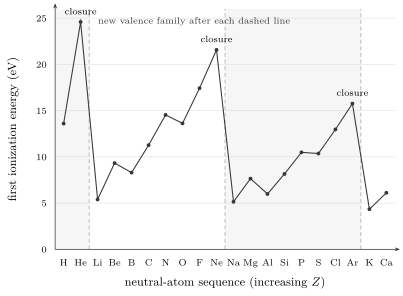
First ionization energies for neutral atoms with , using NIST ASD 5.12 evaluated values. The broad rise across each main-group period and the sharp drops after He, Ne, and Ar reveal periodic shell closure. Local reversals are physical many-electron effects, not measurement noise.
Across the second and third periods, the first ionization energy broadly rises as increasing nuclear charge contracts and binds the valence region. At a noble-gas closure it is relatively large. Adding the next electron begins a more diffuse family, producing the sharp He-to-Li, Ne-to-Na, and Ar-to-K drops.
The pattern is periodic, not monotonic. Four useful local comparisons are:
| Pair and first ionization energies | Main qualitative lesson |
|---|---|
| Be, B: | The first electron in B is easier to remove than a electron from Be. |
| N, O: | Interaction and term energies make removal from easier than a smooth trend predicts. |
| Mg, Al: | The -to- change repeats the Be–B mechanism. |
| P, S: | The half-filled and more-than-half-filled sectors differ in exchange and relaxation energy. |
Orbital penetration gives the first and third comparisons a useful starting intuition. The second and fourth require the many-electron terms of both the neutral atom and its ion. “Paired electrons repel” is too compressed to be a derivation: the measured threshold is a difference of two optimized correlated energies.
Successive ionization and core closure
Section titled “Successive ionization and core closure”Neutral sodium has the leading structure . NIST gives
The large jump does not mean that a classical shell wall has been crossed. After the diffuse electron is removed, the next threshold starts from the compact neon-like ion . Successive ionization energies are therefore a direct empirical probe of changing charge sectors and core closure.
Effective Nuclear Charge and Broad Trends
Section titled “Effective Nuclear Charge and Broad Trends”A one-parameter estimate sometimes writes a valence binding scale as
Here may include a quantum defect, and is fitted or defined within a particular model. The expression is useful for trend reasoning but should not be inverted into a unique experimentally measured effective charge.
Across a main-group period
Section titled “Across a main-group period”As increases while electrons enter the same broad valence shell:
- core screening changes less rapidly than the nuclear charge;
- the valence region generally contracts;
- first ionization energies generally rise;
- static polarizabilities generally fall;
- electron-accepting and bond-polarizing tendencies often increase.
Every “generally” matters. Subshell changes, term structure, correlation, and relativistic effects create local reversals.
Down a group
Section titled “Down a group”Moving down a group introduces a valence orbital with a larger principal radial scale:
- the characteristic atomic size generally grows;
- the outer electron is usually more screened and easier to remove;
- excitation energies often decrease;
- the electron cloud is often more polarizable.
Core penetration and relativistic contraction can weaken or reverse a naive extrapolation. The heavy and sectors, for example, cannot be understood quantitatively by scaling a nonrelativistic hydrogen orbital.
From Atomic Trends to Chemical Trends
Section titled “From Atomic Trends to Chemical Trends”Chemistry compares energies of atoms, ions, molecules, solids, and their environments. An isolated neutral-atom configuration is useful input, but it is not the output of a bonding calculation.
| Trend language | Quantum content and boundary |
|---|---|
| atomic size | Radial density and response of a specified state; no single radius operator equals every tabulated atomic radius. |
| ionization energy | A total-energy difference between charge sectors, not exactly one orbital eigenvalue. |
| electron affinity | An energy difference after attachment; some anions are weakly bound, metastable, or environment-stabilized. |
| electronegativity | A tendency inferred from molecular or thermochemical data; several inequivalent scales exist. |
| polarizability | An induced-dipole response through excited states; it is tensorial and frequency-dependent in general. |
| oxidation state | An electron-counting convention tied to bonding, not a direct isolated-atom observable. |
For a nondegenerate isotropic atomic ground state, the static dipole polarizability has the spectral form
Diffuse valence states and low excitation gaps tend to increase . This helps connect the low first ionization energies of alkali atoms with their large response, but the relation is not an identity: transition matrix elements and the full excited spectrum also matter.
Why groups resemble one another
Section titled “Why groups resemble one another”Elements in a group often present the same number and angular type of low-energy valence electrons outside a compact core. Their valence Hilbert spaces and dominant bonding channels then resemble one another.
The resemblance is approximate because the core changes:
- radial nodes and characteristic length scales differ;
- core polarization and core–valence correlation differ;
- accessible or channels can enter;
- spin–orbit coupling grows;
- oxidation and bonding energies need not scale together.
Group membership is therefore a highly successful structural classification, not a symmetry equivalence between different elements.
Transition and inner-transition trends
Section titled “Transition and inner-transition trends”Partially filled and subshells support many Pauli-allowed terms, several oxidation sectors, and dense low-energy spectra. Their chemistry depends on a competition among:
The lanthanide contraction is associated with increasing nuclear charge across the series combined with incomplete screening by the compact electrons; relativistic effects refine the quantitative trend. It is not evidence that screening disappears.
Why the Explanation Is Approximate
Section titled “Why the Explanation Is Approximate”Periodicity is emergent
Section titled “Periodicity is emergent”The microscopic Hamiltonian does not contain labels such as “group 1,” “halogen,” or “transition metal.” These classifications summarize recurring low-energy behavior after a hierarchy of scales has emerged.
Configurations are basis dependent
Section titled “Configurations are basis dependent”An exact eigenstate can mix configuration-state functions with the same exact and parity. The leading configuration may remain an excellent label, but a percentage attached to it depends on the orbital basis and model space.
Subshell crossings are real
Section titled “Subshell crossings are real”When two configurations are near degenerate, small exchange, correlation, relaxation, or relativistic contributions can change their order. A universal rule cannot encode all of those species-dependent energy differences.
Relativity reshapes heavy atoms
Section titled “Relativity reshapes heavy atoms”The characteristic relativistic parameter grows roughly as
with the fine-structure constant. Direct relativistic contraction is strongest for orbitals with substantial nuclear penetration, especially and spinors, while indirect screening changes can expand other orbitals. Heavy-element trends therefore reflect a coupled relativistic many-electron response.
Chemistry changes the Hamiltonian
Section titled “Chemistry changes the Hamiltonian”In a molecule or solid, spherical symmetry is broken and atomic orbitals hybridize into environment-dependent states. Ionization energies, electron affinities, ligand fields, band formation, and collective screening all participate. Free-atom periodicity remains a guide, not a substitute for solving the new system.
The heaviest elements are a frontier
Section titled “The heaviest elements are a frontier”For short-lived superheavy nuclei, experimental chemistry can be atom-at-a-time and theory must combine relativistic electronic structure with nuclear lifetimes and production constraints. Predictions should be labeled as predictions, and uncertainty should not be hidden behind a familiar group label.
A Reliable Reasoning Workflow
Section titled “A Reliable Reasoning Workflow”When using the periodic table as a quantum-mechanical argument:
- Name the system. Specify the element, isotope if relevant, charge state, and environment.
- Name the observable. Configuration, term, ionization threshold, radius, polarizability, and bond energy are different quantities.
- Separate counting from energetics. Use Pauli for capacities and a Hamiltonian for energy order.
- Choose the reference model. State whether orbitals come from a central field, Hartree–Fock, density-functional, or relativistic calculation.
- Use total-energy differences for thresholds. Include relaxation and correlation at the required accuracy.
- Treat filling rules as proposals. Verify near-degenerate configurations against calculation or evaluated spectroscopy.
- Check the regime. Relativity, open-shell correlation, and chemical environment can change the dominant picture.
- Compare with evaluated data. Preserve reported uncertainties and distinctions between measured, inferred, and calculated values.
This workflow turns a trend into a testable physical statement.
Common Mistakes
Section titled “Common Mistakes”“The nth period contains 2n² elements”
Section titled ““The nth period contains 2n² elements””The number counts all spin-orbitals in an ideal hydrogenic principal shell. Real periods follow interleaved subshell energies; period 3 ends after , while is developed in period 4.
“Pauli determines the filling order”
Section titled ““Pauli determines the filling order””Pauli limits admissible occupations. It does not compare the energies of different admissible configurations.
“Effective nuclear charge is Z minus the number of inner electrons”
Section titled ““Effective nuclear charge is Z minus the number of inner electrons””That may be a rough mnemonic for a selected valence orbital. In a self-consistent atom, screening is radial, orbital dependent, and incomplete in overlapping regions.
“Ionization energy is minus the last orbital energy”
Section titled ““Ionization energy is minus the last orbital energy””This is a model-dependent approximation. The exact threshold is a difference between states with different electron numbers.
“Trends have no exceptions”
Section titled ““Trends have no exceptions””A trend is a coarse-grained pattern. Local reversals encode subshell changes, term energies, relaxation, correlation, and relativity; they are part of the explanation.
“Atoms in one group have the same chemistry”
Section titled ““Atoms in one group have the same chemistry””They share recurring valence structure, not identical Hamiltonians. Radial scale, accessible oxidation sectors, relativistic effects, and environment all evolve down a group.
“A neutral ground configuration specifies bonding”
Section titled ““A neutral ground configuration specifies bonding””Bonding reorganizes the electronic state in the field of other nuclei or a solid. Atomic configurations are inputs and labels, not complete molecular wavefunctions.
Exercises
Section titled “Exercises”Exercise 1: Derive the subshell and shell capacities
Section titled “Exercise 1: Derive the subshell and shell capacities”Show that a nonrelativistic subshell holds electrons. Then sum over to obtain .
Solution
There are possible values of and two values of . Pauli exclusion allows each complete spin-orbital only once, so
Summing the odd integers gives
The result counts a hydrogenic principal shell. It does not determine a period length once interactions split and interleave subshells.
Exercise 2: Why period 3 has eight elements
Section titled “Exercise 2: Why period 3 has eight elements”Hydrogenic counting assigns the shell a capacity of . Explain why the third period nevertheless runs from Na to Ar and has length .
Solution
The hydrogenic shell contains , , and , with capacities
In neutral multi-electron atoms, screening and penetration remove the hydrogenic degeneracy. The valence family becomes relevant before the family is developed across the neutral sequence. Period 3 therefore consists nominally of
with length . The block appears between and in period 4. This is energetic interleaving, not a change in the state capacity of .
Exercise 3: Effective-potential limits
Section titled “Exercise 3: Effective-potential limits”An atom has nuclear charge , bound electrons, and ionic charge . Determine the leading central potential seen by one electron near the nucleus and far outside the other electrons.
Solution
Near the nucleus, the electronic Hartree-like potential is finite for a regular density, while the nuclear attraction is singular:
Far outside, the electron encloses the nucleus and the other electrons. Their net charge is
so
For a neutral atom, and the tail is . The interpolation between these limits is radial and cannot generally be replaced by one constant effective charge.
Exercise 4: Read the local ionization reversals
Section titled “Exercise 4: Read the local ionization reversals”Use the table above to explain why and do not contradict the broad rise across period 2.
Solution
Boron begins the subshell:
The electron penetrates less strongly and is more weakly bound than a electron in the neighboring system, so the first threshold drops at B.
Nitrogen and oxygen both ionize from , but their many-electron terms differ. Nitrogen’s half-filled ground sector is strongly exchange stabilized. Removing one electron from oxygen’s sector produces the favorable ion. The exact comparison is still a difference of separately relaxed total energies; “pairing” is only shorthand for that term, exchange, and correlation balance.
Exercise 5: The sodium jump
Section titled “Exercise 5: The sodium jump”Using the NIST values on this page, compute the ratio for sodium and explain its physical meaning.
Solution
The ratio is
The first ionization removes the diffuse valence electron. The second starts from the compact neon-like ion and removes a core electron. The large ratio is evidence for a change in electronic sector and shell closure, not a literal discontinuity in a classical radial shell.
Exercise 6: Koopmans’ approximation
Section titled “Exercise 6: Koopmans’ approximation”Why can approximate an ionization energy, and what physics does the approximation omit?
Solution
In Hartree–Fock, removing an electron from an occupied canonical orbital while freezing every remaining orbital changes the determinant energy by the negative orbital eigenvalue. This is Koopmans’ construction:
The actual ion relaxes: its orbitals and mean field reoptimize. Correlation energy also differs between the neutral atom and ion. Relativistic, recoil, and radiative effects may matter at higher precision. Thus the exact observable remains
Exercise 7: Similarity without identity
Section titled “Exercise 7: Similarity without identity”Lithium and sodium both have one electron outside a closed core. Give three reasons their atomic or chemical properties are not identical.
Solution
Any three of the following suffice:
- Li uses a valence orbital, while Na uses ; their radial nodes and sizes differ.
- The closed cores have different polarizabilities and core-excitation spectra.
- Their ionization and excitation energies differ.
- Core–valence correlation and exchange differ.
- Relativistic corrections, though modest here, are not identical.
- Molecular bond energies depend on partner atoms and geometry, not only the isolated neutral configuration.
The shared one-valence-electron structure explains family resemblance. It does not define a symmetry mapping one element’s Hamiltonian into the other’s.
Cross-Links
Section titled “Cross-Links”- Multi-Electron Atoms
- Electron Configurations
- Pauli Principle in Atoms
- Hund’s Rules
- Exchange and Correlation
- Hartree Method
- Hartree–Fock for Atoms
- Central-Field Approximation
- Atomic Orbitals Revisited
- Alkali Atoms
- Atomic Term Symbols
- Hydrogen Atom
- AMO Physics Roadmap
References
Section titled “References”- International Union of Pure and Applied Chemistry, Periodic Table of Elements, current table release dated 4 May 2022, accessed 2026-07-21.
- A. Kramida, Yu. Ralchenko, J. Reader, and the NIST ASD Team, NIST Atomic Spectra Database, version 5.12, National Institute of Standards and Technology, 2024, DOI: 10.18434/T4W30F, accessed 2026-07-21.
- NIST Atomic Spectra Database, Ionization Energies Form, critically evaluated ground states and ionization thresholds, accessed 2026-07-21.
- International Union of Pure and Applied Chemistry, “Ionization Energy”, Compendium of Chemical Terminology, 5th ed., online version 5.0.0, 2025.
- W. C. Martin and W. L. Wiese, “Atomic Spectroscopy: An Introduction”, in G. W. F. Drake, ed., Atomic, Molecular, and Optical Physics Handbook, AIP Press, 1996; NIST online revision.
- W. Pauli, “Über den Zusammenhang des Abschlusses der Elektronengruppen im Atom mit der Komplexstruktur der Spektren,” Zeitschrift für Physik 31, 765–783 (1925), doi:10.1007/BF02980631.
- D. R. Hartree, “The Wave Mechanics of an Atom with a Non-Coulomb Central Field. Part I. Theory and Methods,” Proceedings of the Cambridge Philosophical Society 24, 89–110 (1928), doi:10.1017/S0305004100011919.
- V. Fock, “Näherungsmethode zur Lösung des quantenmechanischen Mehrkörperproblems,” Zeitschrift für Physik 61, 126–148 (1930), doi:10.1007/BF01340294.
- J. C. Slater, “Atomic Shielding Constants,” Physical Review 36, 57–64 (1930), doi:10.1103/PhysRev.36.57.
- R. D. Cowan, The Theory of Atomic Structure and Spectra (University of California Press, 1981), especially Chapters 3–8.
- W. R. Johnson, Atomic Structure Theory: Lectures on Atomic Physics (Springer, 2007), doi:10.1007/978-3-540-68013-0.
- C. J. Foot, Atomic Physics (Oxford University Press, 2005), Chapters 3–5.
- B. H. Bransden and C. J. Joachain, Physics of Atoms and Molecules, 2nd ed. (Pearson, 2003), Chapters 6–8.
- P. Pyykkö, “The Physics behind Chemistry and the Periodic Table,” Chemical Reviews 112, 371–384 (2012), doi:10.1021/cr200042e.
- P. Schwerdtfeger, O. R. Smits, and P. Pyykkö, “The Periodic Table and the Physics That Drives It,” Nature Reviews Chemistry 4, 359–380 (2020), doi:10.1038/s41570-020-0195-y.