Helium Atom

Helium is the first atom whose electronic Schrödinger equation contains a genuine interaction between indistinguishable particles. It has only two electrons, yet their Coulomb repulsion prevents exact separation into one-electron problems. Antisymmetry ties spatial exchange to spin, producing distinct singlet and triplet spectra, while explicit dependence on the interelectronic distance is needed for high-accuracy energies.

This combination makes helium unusually valuable. It is simple enough that the nonrelativistic Coulomb problem can be solved numerically to extraordinary precision, but rich enough to expose screening, exchange, correlation, recoil, relativistic effects, radiative corrections, metastability, and spectroscopic selection rules. A method that claims quantitative accuracy for interacting electrons should be able to say exactly which helium quantity it predicts and how that prediction converges.

Canonical Scope and Conventions

This page owns helium as an atomic system: its Hamiltonian hierarchy, state labels, low-lying spectrum, exchange structure, and benchmark role.

The complete one-parameter effective-charge integral is worked through at Variational Estimate for the Helium Atom. General determinant algebra belongs to Slater Determinants, and the generic mean-field derivation belongs to Hartree–Fock Approximation. Here those results are compared as rungs in an atomic approximation hierarchy.

LS Coupling owns the general hierarchy and diagnostics behind the singlet, triplet, and fine-structure labels used here.

Unless stated otherwise:

• energies are in Hartree, $E_{\mathrm h}$;
• distances are in Bohr radii, $a_0$;
• the nucleus has charge $Z=2$;
• the leading Hamiltonian is nonrelativistic with an infinitely massive point nucleus;
• the zero of total electronic energy is a bare nucleus plus two electrons at rest at infinity.

These conventions matter. The clamped-nucleus nonrelativistic ground energy is not itself a measured ionization energy, and neither number should be called “the exact helium energy” without qualification.

Physical System and Hamiltonian

In atomic units, the fixed-nucleus electronic Hamiltonian is

$$\begin{aligned} H_\infty ={}&-\frac{1}{2}\nabla_1^2 -\frac{1}{2}\nabla_2^2\\ &-\frac{2}{r_1} -\frac{2}{r_2} +\frac{1}{r_{12}}, \end{aligned}$$

with

$$r_{12}=|\mathbf r_1-\mathbf r_2|.$$

The first four terms are sums of hydrogenic one-electron operators. The final term couples the electron coordinates. A product

$$\Phi(\mathbf r_1,\mathbf r_2) =\phi_a(\mathbf r_1)\phi_b(\mathbf r_2)$$

can represent independent motion in a chosen field, but it cannot reproduce an arbitrary change in the conditional position of electron 2 when electron 1 moves.

Finite nuclear mass

For an isotope with nuclear mass $M$ measured in electron masses, center-of-mass removal produces an internal nonrelativistic Hamiltonian

$$\begin{aligned} H_M ={}&-\frac{1}{2\mu} \left(\nabla_1^2+\nabla_2^2\right) -\frac{1}{M}\nabla_1\!\cdot\!\nabla_2\\ &-\frac{2}{r_1} -\frac{2}{r_2} +\frac{1}{r_{12}}, \end{aligned}$$

where

$$\mu=\frac{M}{M+1}.$$

The cross derivative is the mass-polarization term. It correlates the electron momenta through nuclear recoil and cannot be reproduced merely by replacing $m_e$ with a reduced mass in two independent hydrogenic equations.

Relativistic, radiative, finite-nuclear-size, and hyperfine terms enter at still finer resolution. For $^{4}\mathrm{He}$ the nucleus has spin zero, whereas $^{3}\mathrm{He}$ has nuclear spin $1/2$ and therefore hyperfine structure. A precision comparison must identify the isotope and every retained correction.

Why Helium Is Not Separable

The hydrogenic Hamiltonian separates in spherical coordinates because each term depends on one electron–nucleus distance. Helium contains three geometrically independent scalar distances,

$$r_1,\qquad r_2,\qquad r_{12}.$$

The law of cosines gives

$$r_{12}^2 =r_1^2+r_2^2 -2r_1r_2\cos\theta_{12},$$

so the repulsion depends on the angle between the electron position vectors as well as their radii. Separating a radial equation for each electron discards precisely this angular and radial correlation.

The problem is sometimes called a three-body Coulomb problem when the nucleus is dynamical. That phrase should not suggest classical chaos or indeterminacy. The stationary Schrödinger equation is a linear eigenvalue problem with well-defined bound states. “Not exactly solvable” means that no closed-form separation comparable to hydrogen is known, not that the spectrum cannot be computed accurately.

Coordinates adapted to correlation

Hylleraas coordinates make the important distances explicit:

$$s=r_1+r_2, \qquad t=r_1-r_2, \qquad u=r_{12}.$$

For the symmetric ground-state spatial function, a useful expansion has the schematic form

$$\Psi(s,t,u) =e^{-\zeta s} \sum_{lmn}c_{lmn}s^l t^{2m}u^n.$$

The powers of $u$ describe direct electron–electron correlation. Even powers of $t$ enforce symmetry under $r_1\leftrightarrow r_2$. This coordinate choice was historically decisive because a modest explicitly correlated expansion could recover effects that require many ordinary orbital products.

Exact and Approximate Quantum Numbers

The spin-independent Hamiltonian $H_\infty$ commutes with

$$L^2,\quad L_z,\quad S^2,\quad S_z, \quad\text{and parity}.$$

Exchange symmetry is also exact. The total electronic state must satisfy

$$P_{12}\Psi_{\mathrm{total}} =-\Psi_{\mathrm{total}}.$$

The nonrelativistic ground state has a positive, symmetric spatial factor with

$$L=0,\qquad \pi=+1.$$

It must therefore be paired with the antisymmetric spin singlet, giving the spectroscopic label

$$1s^2\,{}^1S_0.$$

Spin–orbit and other relativistic terms preserve total $J$ and parity for an isolated atom but make $L$ and $S$ approximate. Helium is light enough that LS Coupling remains an excellent organizing limit for much of the low-lying spectrum.

Independent-Particle Baseline

First remove electron–electron repulsion and write

$$\begin{aligned} H_0&=h(1)+h(2),\\ h(i)&=-\frac{1}{2}\nabla_i^2-\frac{Z}{r_i}. \end{aligned}$$

Each $1s$ electron has energy $-Z^2/2$, so the two-electron ground energy of $H_0$ is

$$E_0^{(0)}=-Z^2.$$

For helium,

$$E_0^{(0)}=-4E_{\mathrm h}.$$

This is not a variational estimate for the full helium Hamiltonian because the expectation value of $1/r_{12}$ has not yet been included. It overbinds the atom severely.

Using the bare $Z=2$ hydrogenic $1s^2$ state as a trial state for the full Hamiltonian gives

$$\left\langle\frac{1}{r_{12}}\right\rangle =\frac{5Z}{8}.$$

Therefore

$$E_{\mathrm{bare}} =-Z^2+\frac{5Z}{8},$$

and for helium

$$E_{\mathrm{bare}}=-2.75E_{\mathrm h}.$$

This is a legitimate variational upper bound. The difference between $-4E_{\mathrm h}$ and $-2.75E_{\mathrm h}$ is not a small correction: electron repulsion reorganizes the orbital scale.

One-Parameter Variational Screening

Let both electrons occupy normalized exponential orbitals with adjustable exponent $\zeta$,

$$\phi_\zeta(r) =\left(\frac{\zeta^3}{\pi}\right)^{1/2} e^{-\zeta r}.$$

Pair the symmetric spatial product with the spin singlet. The energy expectation is

$$E(\zeta) =\zeta^2-2Z\zeta+\frac{5}{8}\zeta.$$

Minimization gives

$$\zeta_\star=Z-\frac{5}{16}.$$

For $Z=2$,

$$\zeta_\star=\frac{27}{16}=1.6875$$

and

$$\begin{aligned} E_{\mathrm{var}} &=-\left(Z-\frac{5}{16}\right)^2\\ &=-\frac{729}{256}E_{\mathrm h}\\ &=-2.84765625E_{\mathrm h}. \end{aligned}$$

The exponent is smaller than the true nuclear charge because each electron screens the nucleus for the other on average. This one number captures radial relaxation but not an instantaneous dependence on $r_{12}$. The full evaluation of the Coulomb integral and the variational bound is kept at Variational Estimate for the Helium Atom.

What the trial state means

The probability density factorizes:

$$|\Psi_\zeta(\mathbf r_1,\mathbf r_2)|^2 =|\phi_\zeta(r_1)|^2 |\phi_\zeta(r_2)|^2.$$

Knowing electron 1’s position therefore does not change the conditional spatial distribution of electron 2. The optimized exponent accounts for average screening, but it cannot describe the electrons avoiding one another differently on opposite sides of the nucleus.

An Energy Ladder

The following values all refer to the fixed-nucleus nonrelativistic Coulomb problem unless noted otherwise.

Description	Ground energy in $E_{\mathrm h}$	What changes
noninteracting $H_0$ eigenvalue	$-4.000000$	omits $1/r_{12}$ entirely; not an upper bound for $H_\infty$
bare $1s^2$ expectation	$-2.750000$	includes repulsion without orbital relaxation
one-exponent variational state	$-2.847656$	optimizes average radial screening
Hartree–Fock limit	approximately $-2.861680$	optimizes a single determinant
correlated Schrödinger value	approximately $-2.903724377034$	converges the two-electron Coulomb eigenproblem

The conventional nonrelativistic correlation energy is

$$\begin{aligned} E_{\mathrm{corr}} &=E_{\mathrm{nr}}-E_{\mathrm{HF}}\\ &\simeq-0.04204438E_{\mathrm h}. \end{aligned}$$

Its magnitude is about $1.14\,\mathrm{eV}$, but that does not mean every helium observable has a one-electron-volt Hartree–Fock error. Energy differences can contain cancellations, and transition amplitudes probe different aspects of the wavefunction.

Total energy versus ionization energy

For the same infinite-mass nonrelativistic Hamiltonian, the residual ion $\mathrm{He}^+$ has

$$E_{\mathrm{nr}}(\mathrm{He}^+)=-2E_{\mathrm h}.$$

The theoretical first ionization energy is therefore

$$\begin{aligned} I_{\mathrm{nr}} &=E_{\mathrm{nr}}(\mathrm{He}^+) -E_{\mathrm{nr}}(\mathrm{He})\\ &\simeq0.903724377E_{\mathrm h} \simeq24.5916\,\mathrm{eV}. \end{aligned}$$

The NIST Atomic Spectra Database gives the physical He I ionization energy as

$$I_{\mathrm{exp}} =24.587389011(25)\,\mathrm{eV}.$$

The few-millielectron-volt difference is expected: finite nuclear mass, relativistic dynamics, QED, and nuclear structure change the idealized Hamiltonian. Comparing $-2.903724E_{\mathrm h}$ directly with $24.587389\,\mathrm{eV}$ would also compare quantities with different energy zeros.

Singlet and Triplet States

For two distinct orthonormal spatial orbitals $a$ and $b$, define exchange-symmetrized spatial functions

$$\begin{aligned} \psi_\pm(1,2) ={}&\frac{1}{\sqrt2}\bigl[ \phi_a(1)\phi_b(2) \\ &\quad\pm\phi_b(1)\phi_a(2)\bigr]. \end{aligned}$$

The plus state is spatially symmetric and must multiply the antisymmetric spin singlet,

$$\chi_{00} =\frac{1}{\sqrt2} \left( \alpha(1)\beta(2) -\beta(1)\alpha(2) \right).$$

The minus state is spatially antisymmetric and must multiply one of the symmetric triplet spin functions,

$$\begin{aligned} \chi_{11}&=\alpha(1)\alpha(2),\\ \chi_{10}&=\frac{1}{\sqrt2} \left[ \alpha(1)\beta(2) +\beta(1)\alpha(2) \right],\\ \chi_{1,-1}&=\beta(1)\beta(2). \end{aligned}$$

If $a=b$, the antisymmetric spatial function vanishes. Two electrons in the same spatial orbital can therefore form the $1s^2$ ground configuration only as a spin singlet.

Direct and exchange splitting

For fixed orthonormal orbitals and a spin-independent Hamiltonian, write the direct and exchange Coulomb integrals as

$$J_{ab} =\iint \frac{|\phi_a(\mathbf r_1)|^2 |\phi_b(\mathbf r_2)|^2} {r_{12}} \,d^3r_1\,d^3r_2$$

and

$$\begin{aligned} K_{ab} ={}&\iint \phi_a^*(\mathbf r_1)\phi_b(\mathbf r_1) \\ &\quad\times \frac{\phi_b^*(\mathbf r_2)\phi_a(\mathbf r_2)} {r_{12}} \,d^3r_1\,d^3r_2. \end{aligned}$$

The spatial energies have the schematic form

$$\begin{array}{ccl} E_{\mathrm{singlet}} &=&h_{aa}+h_{bb}+J_{ab}+K_{ab},\\ E_{\mathrm{triplet}} &=&h_{aa}+h_{bb}+J_{ab}-K_{ab}. \end{array}$$

Thus the fixed-orbital splitting is

$$E_{\mathrm{singlet}}-E_{\mathrm{triplet}} =2K_{ab}.$$

This explains why the triplet member of a given helium configuration often lies lower. It does not make exchange a classical attractive force. The result follows from evaluating the same Coulomb Hamiltonian in spatial states with different exchange symmetry. Orbital relaxation and correlation modify the quantitative splitting.

Historically the singlet system was called parahelium and the triplet system orthohelium. Modern notation states $S$ and the term symbol directly.

Low-Lying Spectrum

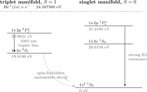
Selected low-lying $^{4}\mathrm{He}$ levels relative to the $1s^2\,{}^1S_0$ ground state, using NIST evaluated energies. The vertical scale is schematic and contains a break between the ground and excited manifolds. The strong singlet resonance and the $1083\,\mathrm{nm}$ triplet transition are electric-dipole allowed; decay from $1s\,2s\,{}^3S_1$ to the singlet ground state is strongly suppressed.

Representative evaluated excitation energies are:

Configuration and level	Excitation energy
$1s\,2s\,{}^3S_1$	$19.819615\,\mathrm{eV}$
$1s\,2s\,{}^1S_0$	$20.615775\,\mathrm{eV}$
$1s\,2p\,{}^3P^\circ_J$	about $20.9641\,\mathrm{eV}$
$1s\,2p\,{}^1P^\circ_1$	$21.218023\,\mathrm{eV}$
$\mathrm{He}^+(1s)+e^-$ limit	$24.587389011\,\mathrm{eV}$

The triplet $2\,{}^3P^\circ_J$ entry contains the fine-structure levels $J=0,1,2$; the schematic figure does not resolve their much smaller splitting. The singlet–triplet separation within a configuration is primarily electrostatic exchange at this scale, whereas the $J$ splitting within a triplet term is relativistic.

Spectral series

Excited levels form singlet and triplet Rydberg series converging to the same $\mathrm{He}^+(1s)$ threshold. A useful effective description is

$$E_{n\ell S} \simeq I_{\mathrm{He}} -\frac{R_{\mathrm{He}}} {(n-\delta_{\ell S})^2},$$

where the quantum defect $\delta_{\ell S}$ depends on orbital penetration, exchange symmetry, and core polarization. The outer electron becomes hydrogenic at large radius, but the residual core is a polarizable $\mathrm{He}^+$ ion rather than an inert point charge.

Selection Rules and Metastability

The leading electric-dipole operator is odd under parity and does not act on spin. In the $LS$ limit, an E1 transition therefore requires

$$\Delta S=0, \qquad \pi_f=-\pi_i,$$

together with the usual angular-momentum rule

$$\Delta J=0,\pm1, \qquad J=0\not\leftrightarrow J=0.$$

Consequences for helium include:

• $1s\,2p\,{}^1P^\circ_1\rightarrow1s^2\,{}^1S_0$ is a strong resonance transition near $58.4\,\mathrm{nm}$.
• $1s\,2p\,{}^3P^\circ_J\rightarrow1s\,2s\,{}^3S_1$ produces the important triplet line near $1083\,\mathrm{nm}$.
• $1s\,2s\,{}^1S_0\rightarrow1s^2\,{}^1S_0$ is E1-forbidden by parity and the $0\leftrightarrow0$ rule, but two-photon decay is allowed.
• $1s\,2s\,{}^3S_1\rightarrow1s^2\,{}^1S_0$ changes spin and has no parity change, so its leading E1 amplitude vanishes.

The $2\,{}^3S_1$ level is consequently metastable, with a natural lifetime of order $10^4\,\mathrm{s}$. Weak relativistic magnetic and spin-mixing mechanisms eventually permit decay. Its long lifetime and the accessible $1083\,\mathrm{nm}$ cycling transition make metastable helium a useful AMO platform, but the metastability is an approximate selection-rule consequence rather than an exact superselection law.

The tensor-operator derivation and convention checks belong to Atomic Selection Rules.

Correlation Beyond a Single Determinant

For the $1s^2$ singlet, a restricted Hartree–Fock wavefunction is one determinant built from a doubly occupied spatial orbital. It enforces total antisymmetry and optimizes the orbital self-consistently. It does not permit the spatial state to respond explicitly to the instantaneous value of $r_{12}$.

Hartree–Fock for Atoms derives why this two-electron closed-shell equation coincides with the optimized spatial Hartree equation while still omitting the explicit Coulomb correlation represented below.

An explicitly correlated ansatz may contain a factor such as

$$\begin{aligned} \Psi_{\mathrm{corr}} ={}&e^{-\zeta(r_1+r_2)} \bigl(1+c_1r_{12}\\ &\quad+c_2r_{12}^2+\cdots\bigr). \end{aligned}$$

When one electron approaches the other, the $r_{12}$ dependence adjusts the local slope. For opposite-spin electron coalescence, the spherical-average Kato cusp condition is

$$\left. \frac{1}{\Psi} \frac{\partial\Psi}{\partial r_{12}} \right|_{r_{12}=0} =\frac{1}{2}.$$

At electron–nucleus coalescence for an infinitely massive point nucleus,

$$\left. \frac{1}{\Psi} \frac{\partial\Psi}{\partial r_i} \right|_{r_i=0} =-Z.$$

Ordinary finite orbital expansions converge slowly near these nonanalytic cusps. Hylleraas, explicitly correlated Gaussian, and $R_{12}/F_{12}$-type methods build interelectronic distances or cusp information more directly into the representation.

Dynamic and angular correlation

Two complementary pictures are useful:

• Radial correlation: when one electron lies unusually close to the nucleus, the other tends to occupy a more diffuse radial region.
• Angular correlation: electrons preferentially occupy different directions around the nucleus, increasing their average separation.

These are interpretations of the pair density, not assignments of persistent identities to “inner” and “outer” electrons. The exact state remains exchange symmetric in its spatial coordinates.

Helium as a Computational Benchmark

Helium benchmarks more than one final energy. It tests whether a method can represent:

1. the electron–nucleus and electron–electron cusps;
2. antisymmetry and spin adaptation;
3. diffuse Rydberg orbitals and continuum thresholds;
4. singlet–triplet exchange splittings;
5. relativistic fine structure;
6. recoil and isotope dependence;
7. QED corrections and transition amplitudes.

Method ladder

Method	Helium use	Main diagnostic
one-parameter variational	screening and upper-bound logic	analytic energy minimum
Hartree–Fock	optimized independent-particle reference	self-consistency, virial ratio, basis limit
configuration interaction	orbital expansion of correlation	excitation-rank and angular-basis convergence
Hylleraas or explicitly correlated basis	high-precision few-electron states	cusp behavior and nonlinear-parameter stability
many-body perturbation or coupled cluster	method benchmarking in a minimal atom	order or truncation convergence
quantum Monte Carlo	stochastic correlation treatment	variance, time-step, population, and nodal errors
nonrelativistic QED expansion	precision level and isotope comparisons	order-by-order uncertainty budget

The same numerical value can arise from compensating errors. A robust benchmark reports several diagnostics.

Virial theorem

For an exact stationary state of a Coulomb Hamiltonian,

$$2\langle T\rangle+\langle V\rangle=0.$$

A variational energy may look converged while violating this relation noticeably. The virial residual is therefore a useful independent check, especially when nonlinear scale parameters have not been fully optimized.

Energy variance and residual

For a normalized approximate state,

$$\sigma_H^2 =\langle H^2\rangle-\langle H\rangle^2 =\|(H-E)\Psi\|^2,$$

with $E=\langle H\rangle$. An exact eigenstate has zero variance. Small energy error does not guarantee a uniformly accurate local wavefunction, so cusp checks, expectation values, transition matrix elements, and residual norms add information.

Layered precision theory

A precision calculation should be organized as

$$\begin{aligned} E_{\mathrm{theory}} ={}&E_{\mathrm{nr}}^{(\infty)} +\delta E_{\mathrm{mass}} +\delta E_{\mathrm{rel}}\\ &+\delta E_{\mathrm{QED}} +\delta E_{\mathrm{nuc}} +\cdots . \end{aligned}$$

Each term needs a declared isotope, constants adjustment, and uncertainty estimate. Agreement with experiment at one level of this hierarchy does not validate omitted higher-order terms.

Experimental and Data Practice

The NIST Atomic Spectra Database is the appropriate starting point for critically evaluated He I energies, wavelengths, transition probabilities, and ionization energies. Its current ionization-energy entry provides an uncertainty and source reference; the older Handbook of Basic Atomic Spectroscopic Data remains useful for a compact level table.

For a reproducible comparison:

• identify He I rather than He II;
• state $^{3}\mathrm{He}$ or $^{4}\mathrm{He}$;
• distinguish excitation energy from total binding and first ionization energy;
• preserve the reported uncertainty and significant figures;
• distinguish observed wavelengths from Ritz wavelengths derived from optimized levels;
• state whether the calculation is nonrelativistic, relativistic, or NRQED;
• compare values with the same energy zero and constants convention.

Helium’s apparent simplicity makes convention errors more visible, not less consequential.

Common Mistakes

Calling the noninteracting value a variational energy

$-4E_{\mathrm h}$ is the eigenvalue of $H_0$ after deleting electron repulsion. The expectation of the full Hamiltonian in the same orbitals is $-2.75E_{\mathrm h}$.

Treating the optimized exponent as the measured nuclear charge

The nucleus still has $Z=2$. The value $\zeta=27/16$ is a parameter in one chosen trial family that summarizes average screening.

Saying Hartree–Fock omits exchange

Hartree–Fock includes exchange exactly within a single determinant. It omits correlation beyond that determinant.

Assigning one electron permanently to each orbital

The labels 1 and 2 are coordinate slots. In an antisymmetrized $1s\,2s$ state there is no observable fact about which persistent electron is “the $1s$ electron.”

Using singlet and triplet as parity labels

Singlet and triplet specify $S=0$ and $S=1$. Parity follows from the orbital angular momenta and must be tracked separately.

Comparing a total energy with an ionization energy

The total ground energy uses the bare nucleus plus two free electrons as zero. The first ionization energy is a difference between neutral helium and $\mathrm{He}^+$.

Calling a forbidden transition impossible

“E1-forbidden in the nonrelativistic $LS$ limit” does not mean exactly zero in the full theory. Higher multipoles, two-photon processes, relativistic mixing, external fields, and collisions can open weak channels.

Exercises

Exercise 1: Bare independent-particle estimate

For two hydrogenic $1s$ orbitals with nuclear charge $Z$, use

$$\left\langle\frac{1}{r_{12}}\right\rangle =\frac{5Z}{8}$$

to find the expectation of the full two-electron Hamiltonian. Evaluate it for helium and explain why it is an upper bound.

Solution

The two one-electron energies sum to $-Z^2$. Adding the repulsion expectation gives

$$E_{\mathrm{bare}} =-Z^2+\frac{5Z}{8}.$$

For $Z=2$,

$$E_{\mathrm{bare}} =-4+\frac{10}{8} =-2.75E_{\mathrm h}.$$

The normalized $1s^2$ spatial product paired with the spin singlet is an admissible trial state for the full fixed-nucleus Hamiltonian. The variational principle therefore makes its expectation an upper bound to the nonrelativistic ground energy.

Exercise 2: Optimize the screening exponent

Minimize

$$E(\zeta) =\zeta^2-2Z\zeta+\frac{5}{8}\zeta$$

for general $Z$. Evaluate the result for helium and verify the virial relation within this uniformly scaled trial family.

Solution

Differentiating gives

$$\frac{dE}{d\zeta} =2\zeta-2Z+\frac{5}{8}.$$

Hence

$$\zeta_\star=Z-\frac{5}{16}.$$

For helium, $\zeta_\star=27/16$ and

$$E(\zeta_\star) =-\left(\frac{27}{16}\right)^2 =-\frac{729}{256}E_{\mathrm h}.$$

The kinetic expectation is $T=\zeta^2$, while the total Coulomb potential is

$$V=-2Z\zeta+\frac{5}{8}\zeta.$$

At the stationary point, $2\zeta_\star=2Z-5/8$, so

$$\begin{aligned} 2T+V ={}&2\zeta_\star^2 -2Z\zeta_\star\\ &+\frac{5}{8}\zeta_\star =0. \end{aligned}$$

Exercise 3: Exchange symmetry and the ground state

Show that two electrons occupying the same spatial orbital cannot form a triplet. Why does this force the $1s^2$ helium ground configuration to be a singlet?

Solution

The antisymmetric spatial combination of one orbital $\phi$ with itself is

$$\frac{1}{\sqrt2} \left[ \phi(1)\phi(2)-\phi(2)\phi(1) \right]=0.$$

A triplet spin function is symmetric, so fermionic antisymmetry would require precisely this antisymmetric spatial factor. No nonzero triplet state exists with both electrons in the same spatial orbital. The $1s^2$ ground configuration instead has a symmetric spatial product and must multiply the antisymmetric spin singlet, giving $^{1}S_0$.

Exercise 4: Direct and exchange energies

For two distinct orthonormal orbitals, suppose $K_{ab}>0$. Compare the fixed-orbital singlet and triplet energies and explain why this is not evidence for a new exchange force.

Solution

The energies are

$$E_S=h_{aa}+h_{bb}+J_{ab}+K_{ab}$$

and

$$E_T=h_{aa}+h_{bb}+J_{ab}-K_{ab}.$$

Therefore

$$E_S-E_T=2K_{ab}>0.$$

The triplet lies lower in this fixed-orbital model. Both energies are expectations of the same kinetic, nuclear-attraction, and Coulomb-repulsion Hamiltonian. Their difference arises because antisymmetry changes the spatial interference and pair density; no additional classical force has been introduced.

Exercise 5: Ionization energies and Hamiltonian layers

Using $E_{\mathrm{nr}}(\mathrm{He})=-2.903724377E_{\mathrm h}$ and $E_{\mathrm{nr}}(\mathrm{He}^+)=-2E_{\mathrm h}$, find the nonrelativistic infinite-mass ionization energy in Hartree. Why does its conversion to electronvolts not exactly equal the NIST physical value?

Solution

The threshold difference is

$$\begin{aligned} I_{\mathrm{nr}} &=-2E_{\mathrm h} -(-2.903724377E_{\mathrm h})\\ &=0.903724377E_{\mathrm h}. \end{aligned}$$

Using the stated Hartree conversion gives approximately $24.5916\,\mathrm{eV}$. The NIST value describes physical helium and includes finite nuclear mass, relativistic, radiative, and nuclear effects absent from the idealized Hamiltonian. The discrepancy is therefore not simply numerical error in the correlated Schrödinger calculation.

Exercise 6: Classify helium decays

Classify each transition at leading E1 order:

1. $1s\,2p\,{}^1P^\circ_1\rightarrow1s^2\,{}^1S_0$;
2. $1s\,2s\,{}^1S_0\rightarrow1s^2\,{}^1S_0$;
3. $1s\,2s\,{}^3S_1\rightarrow1s^2\,{}^1S_0$;
4. $1s\,2p\,{}^3P^\circ_1\rightarrow1s\,2s\,{}^3S_1$.

Solution

1. Allowed: parity changes, $\Delta S=0$, and $J=1\rightarrow0$.
2. Forbidden at E1 order: parity does not change and $J=0\rightarrow0$. Two-photon decay can occur.
3. Forbidden at E1 order: parity does not change and $\Delta S=1$. Weak higher-order decay remains possible.
4. Allowed: parity changes, $\Delta S=0$, and $J=1\rightarrow1$ satisfies the angular-momentum rule.

The classification names the leading multipole approximation. It does not declare the forbidden channels exactly absent in the full Hamiltonian.

Cross-Links

• Multi-Electron Atoms
• Atomic Correlation Methods Overview
• Electron Configurations
• Pauli Principle in Atoms
• Exchange and Correlation
• Hartree Method
• Hartree–Fock for Atoms
• LS Coupling
• Hydrogen as Atomic Prototype
• Atomic Term Symbols
• Atomic Selection Rules
• Variational Estimate for the Helium Atom
• Variational Principle
• Spin and Spatial Wavefunctions
• Pauli Exclusion Principle
• Slater Determinants
• Hartree–Fock Approximation
• Angular Momentum Coupling Schemes
• Atomic Units
• AMO Physics Roadmap

References

1. A. Kramida, Yu. Ralchenko, J. Reader, and the NIST ASD Team, NIST Atomic Spectra Database, version 5.12, National Institute of Standards and Technology, 2024, DOI: 10.18434/T4W30F, accessed 2026-07-21.
2. J. E. Sansonetti and W. C. Martin, “Energy Levels of Neutral Helium (He I)”, Handbook of Basic Atomic Spectroscopic Data, NIST, accessed 2026-07-21.
3. W. C. Martin and W. L. Wiese, “Helium and Helium-Like Ions; LS Coupling”, in Atomic Spectroscopy: An Introduction, NIST, 1996 online edition.
4. H. A. Bethe and E. E. Salpeter, Quantum Mechanics of One- and Two-Electron Atoms, Springer, 1957.
5. E. A. Hylleraas, “Neue Berechnung der Energie des Heliums im Grundzustande, sowie des tiefsten Terms von Ortho-Helium,” Zeitschrift für Physik 54, 347–366 (1929), DOI: 10.1007/BF01375457.
6. C. L. Pekeris, “Ground State of Two-Electron Atoms,” Physical Review 112, 1649–1658 (1958), DOI: 10.1103/PhysRev.112.1649.
7. C. Schwartz, “Ground State of the Helium Atom,” Physical Review 128, 1146–1148 (1962), DOI: 10.1103/PhysRev.128.1146.
8. H. Nakashima and H. Nakatsuji, “How Accurately Does the Free Complement Wave Function of a Helium Atom Satisfy the Schrödinger Equation?” Physical Review Letters 101, 240406 (2008), DOI: 10.1103/PhysRevLett.101.240406.
9. G. W. F. Drake, “High Precision Calculations for Helium,” in G. W. F. Drake, ed., Springer Handbook of Atomic, Molecular, and Optical Physics, Springer, 2006.
10. T. Kato, “On the Eigenfunctions of Many-Particle Systems in Quantum Mechanics,” Communications on Pure and Applied Mathematics 10, 151–177 (1957), DOI: 10.1002/cpa.3160100201.
11. A. Szabo and N. S. Ostlund, Modern Quantum Chemistry: Introduction to Advanced Electronic Structure Theory, Dover, 1996.
12. W. R. Johnson, Atomic Structure Theory: Lectures on Atomic Physics, Springer, 2007.