Electron Configurations
An electron configuration records how the electrons of an atom or ion are distributed among a chosen set of one-electron orbitals or subshells. A familiar example is
This notation is powerful because it compresses electron counting, shell structure, parity, and the starting point for angular-momentum coupling into one line. It is also easy to overread. A configuration is generally not a complete wavefunction, not an observable partition into named electrons, and not necessarily an exact label of an energy eigenstate.
The safest interpretation is:
A configuration is an occupation pattern relative to a declared one-electron basis and coupling convention.
That basis may come from a central-field model, Hartree–Fock calculation, relativistic self-consistent field, or another orbital construction. Residual interactions can mix several configurations into one physical level, and rotating the orbitals can change the reported configuration weights without changing the many-electron state.
Canonical Scope
Section titled “Canonical Scope”This page owns the atomic use of configuration notation: shells and subshells, occupation exponents, compact core notation, the limited logic behind Aufbau filling, closed shells and valence spaces, and the interpretation of mixed configurations.
Hund’s Rules begins only after a configuration and its Pauli-allowed terms have been identified: it approximately ranks those terms and their fine-structure levels, but it does not determine the configuration itself.
Periodic Table from Quantum Mechanics uses configuration patterns as one layer in the explanation of periods, blocks, ionization energies, and broad chemical trends; it does not turn the Aufbau mnemonic into an exact law.
The underlying pieces have canonical homes elsewhere:
- Atomic Orbitals Revisited distinguishes exact one-electron states, basis orbitals, mean-field orbitals, and natural orbitals.
- Occupation-Number Basis develops mode occupations independently of atomic notation.
- Pauli Exclusion Principle derives the allowed fermionic occupations.
- Pauli Principle in Atoms applies antisymmetry to equivalent-electron terms, closed subshells, and periodic shell filling.
- Slater Determinants owns determinant construction and antisymmetry.
- Slater Determinants in Atoms owns the atomic passage from spin-orbital determinants to projection sectors and configuration-state functions.
- Atomic Term Symbols develops the terms and levels supported by a configuration.
- jj Coupling develops relativistic-subshell occupations, parent angular momenta, and their relation to LS labels.
- Central-Field Approximation explains how the reference orbitals and approximate subshell ordering arise.
Here those ingredients are assembled into a reliable language for reading atomic structure calculations and spectroscopic data.
Species, Charge, and Electron Count
Section titled “Species, Charge, and Electron Count”Begin with the number of electrons. For nuclear charge and ionic charge , where denotes a positive ion,
Every proposed configuration must contain exactly electrons. In atomic spectroscopy, a Roman numeral convention is also common:
| Spectroscopic label | Charge | Example |
|---|---|---|
| I | C I is neutral carbon | |
| II | C II is singly ionized carbon | |
| III | C III is doubly ionized carbon |
Thus the Roman numeral is the ion charge plus one. It does not count valence electrons or specify an excitation level.
Electron counting is elementary but diagnostic. A configuration with the wrong total occupation cannot be rescued by a term label, coupling scheme, or correlation correction.
Shells, Subshells, and Spin-Orbitals
Section titled “Shells, Subshells, and Spin-Orbitals”In a nonrelativistic central field, a spatial orbital can be labeled
with principal or radial label , orbital angular momentum , and projection . Including a spin basis gives a spin-orbital
The coordinate includes space and spin. A subshell groups all spin-orbitals with the same and . It contains
spin-orbitals, so its occupation obeys
The familiar capacities follow immediately:
| Subshell | Spatial orbitals | Spin-orbitals | Maximum occupation | |
|---|---|---|---|---|
| 0 | 1 | 2 | 2 | |
| 1 | 3 | 6 | 6 | |
| 2 | 5 | 10 | 10 | |
| 3 | 7 | 14 | 14 |
These are exact dimension counts for the declared one-electron basis. They do not determine the energetic order of the subshells.
Shell language is context dependent
Section titled “Shell language is context dependent”For the Coulomb one-electron problem, all orbitals with the same share an energy before fine structure and radiative corrections. It is then natural to call the complete set of states the th shell, whose capacity is
In a multi-electron central field, screening and penetration lift the hydrogenic degeneracy between different values. Atomic spectroscopy therefore often uses shell loosely for groups such as , while actual calculations organize orbitals by subshell or relativistic spinor. The word should not be used to imply an exact degeneracy that the Hamiltonian does not possess.
Relativistic subshells
Section titled “Relativistic subshells”When spin–orbit structure is built into the one-electron basis, a subshell is commonly labeled or by the Dirac angular quantum number . A fixed- subshell contains
magnetic spinors. Thus a nonrelativistic subshell separates into and subshells of capacities and . Configuration labels must therefore be read together with the coupling convention used to define them.
jj Coupling shows how these occupations are antisymmetrized, coupled to total , and tested as approximate labels of real atomic levels.
Occupation Notation
Section titled “Occupation Notation”For subshells indexed by , a nonrelativistic configuration may be written schematically as
The product sign is symbolic: it lists occupations and is not multiplication of wavefunctions. In a chosen spin-orbital basis, the same subshell occupation is
where every fermionic mode has or . The subshell exponent may exceed one because it sums distinct complete spin-orbitals.
Full and compact forms
Section titled “Full and compact forms”Neutral carbon has six electrons. Its commonly used ground-configuration label is
The bracketed helium symbol abbreviates the filled core. It does not insert a literal helium atom inside carbon. Similarly,
An exponent of one is often omitted, so means . The order in which subshells are printed is conventional. It may emphasize principal shell, spectroscopic ancestry, or an Aufbau mnemonic; it is not by itself a measured ordering of orbital energies.
What a configuration fixes
Section titled “What a configuration fixes”A declared configuration fixes:
- the total number of electrons;
- the occupation of each listed subshell;
- the maximum determinant space compatible with those occupations;
- the configuration parity in a parity-adapted central-field basis.
Its parity is
Closed subshells contribute even parity, so only open subshells need to be inspected in most practical examples.
What a configuration omits
Section titled “What a configuration omits”A configuration does not generally fix:
- which and spin-orbitals are occupied in a determinant;
- how determinants are combined to enforce total , , , or parity;
- which term or fine-structure level is intended;
- the radial form of the orbitals;
- the coefficients of other configurations in the physical state.
For example, is not one state. The subshell contains six spin-orbitals, and choosing two gives
determinants before symmetry adaptation. Their decomposition into allowed terms belongs to Atomic Term Symbols.
More generally, if occupations in distinct subshells are , the number of spin-orbital determinants associated with the configuration is
This count is a basis dimension, not an energy degeneracy after all interactions are included.
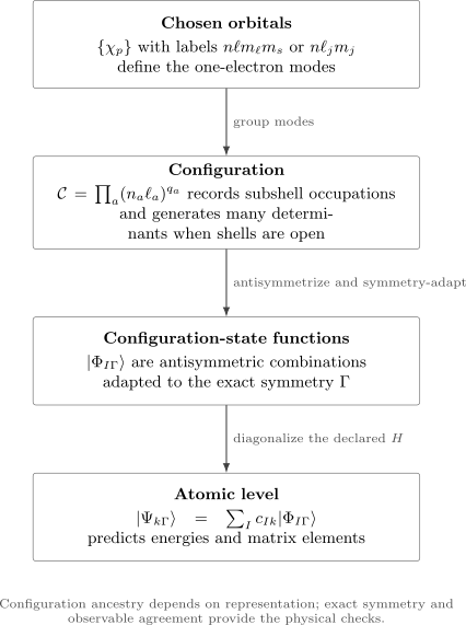
Orbitals define the occupation labels. A configuration generates determinants, which can be combined into configuration-state functions of fixed exact symmetry . Diagonalizing the declared Hamiltonian then mixes all retained functions with that symmetry. Only the final eigenvector is the state predicted by the calculation; every intermediate label depends on representation choices.
Determinants, Configuration-State Functions, and Levels
Section titled “Determinants, Configuration-State Functions, and Levels”Three layers are often compressed into one informal phrase.
Slater Determinants in Atoms develops the transformation among these layers in detail, including determinant phases and symmetry adaptation.
Determinant
Section titled “Determinant”A Slater determinant specifies occupation of complete spin-orbitals. In creation-operator notation,
with a fixed ordering convention. It is antisymmetric by construction. An open-subshell configuration usually generates many such determinants.
Configuration-state function
Section titled “Configuration-state function”A configuration-state function, or CSF, is a symmetry-adapted linear combination of determinants:
The label collects exact symmetries imposed in the calculation. For a field-free rotationally invariant atom it commonly includes and parity. In a nonrelativistic electrostatic calculation it may also include separately conserved and .
Atomic level
Section titled “Atomic level”An approximate eigenstate in the retained CSF space is
Several CSFs may come from one configuration, and several configurations may contribute CSFs with the same . A level label such as a principal configuration and term identifies the dominant ancestry of this eigenvector; it does not replace the eigenvector.
The Aufbau Principle as a Conditional Result
Section titled “The Aufbau Principle as a Conditional Result”The German word Aufbau means building up. In its careful form, the principle says that a reference configuration can be constructed by occupying low-energy one-electron states subject to Pauli exclusion. This statement is exact for a fixed noninteracting reference Hamiltonian and only heuristic for an interacting self-consistent atom.
Consider
An occupation-number eigenstate has energy
Suppose , mode is occupied, and mode is empty. Exchanging their occupations changes the energy by
Therefore the ground state of this fixed occupies the lowest spin-orbitals. That exchange argument is the precise theorem behind the elementary filling rule.
Why the theorem does not settle real atoms
Section titled “Why the theorem does not settle real atoms”The electronic Hamiltonian also contains two-electron interactions:
In a self-consistent model, even the orbitals and their values depend on which states are occupied. The pair interaction adds direct and exchange energies that are not a sum of fixed one-electron numbers, and the residual Hamiltonian mixes configurations. Relativistic shifts, core relaxation, and correlation add further state dependence.
Consequently, these are different questions:
- Which orbital is lower in a chosen one-electron reference potential?
- Which configuration minimizes a self-consistent total energy for a specified atom or ion?
- Which electron-removal channel gives the lowest ionization threshold?
- Which configuration is the largest component of the exact or calculated eigenstate?
They need not have the same answer.
The Madelung Ordering and Its Limits
Section titled “The Madelung Ordering and Its Limits”The common or Madelung rule orders subshells by increasing , breaking ties by lower . It gives the mnemonic sequence beginning
For many neutral ground configurations this is an efficient memory aid. Its qualitative basis is that penetration and screening split subshells that would be degenerate in a hydrogenic model. It is not an eigenvalue theorem for the many-electron Coulomb Hamiltonian.
Several limitations matter:
- The order depends on nuclear charge, ionic charge, and occupation.
- Nearby and subshells can reorder as electrons are added or removed.
- Direct Coulomb, exchange, and radial-relaxation energies belong to the total configuration, not to a universal list of orbital boxes.
- Spin–orbit and other relativistic effects become increasingly important for heavy atoms.
- Near-degenerate configurations may mix so strongly that one filling string is an incomplete description.
Neutral chromium and copper are familiar warnings. Their commonly assigned leading ground configurations are
rather than the simplest uncorrected Madelung predictions. Saying only that half-filled or filled subshells are “especially stable” is not a calculation. The energy balance includes all direct, exchange, relaxation, relativistic, and correlation contributions for the species under study.
Ionization supplies another warning. In first-row transition atoms, can be occupied before substantial filling in the neutral sequence, yet occupation is commonly lost first upon ionization. The reference potential and orbital ordering have changed. “Last filled” is not a general theorem for “first removed.”
For actual assignments, use evaluated level data rather than repairing the mnemonic with a longer exception list. The NIST Atomic Spectra Database separates ground shells, principal configurations, levels, energies, and uncertainties for atoms and ions.
Closed Subshells and Closed-Shell States
Section titled “Closed Subshells and Closed-Shell States”A nonrelativistic subshell is closed when
Every value then occurs with both spin projections. The filled determinant is invariant under rotations within the complete subshell, so it carries
Its parity is even because
A configuration composed entirely of closed nonrelativistic subshells therefore supports a state. In a relativistic description, a completely filled subshell likewise contributes total .
Closed subshell is not synonymous with noble gas
Section titled “Closed subshell is not synonymous with noble gas”The phrases closed subshell, closed shell, and noble-gas core answer different questions.
- is a closed subshell.
- abbreviates a particular collection of closed subshells.
- contains a closed subshell but is not a noble-gas configuration.
- A “closed-shell core” is a modeling partition between orbitals treated as core and those treated as active or valence.
Closed angular-momentum coupling does not make a core physically inert. Core orbitals can relax between states, polarize in the field of a valence electron, contribute to exchange, and participate through virtual or real core excitations.
Valence Electrons and Active Spaces
Section titled “Valence Electrons and Active Spaces”In the simplest atomic language, valence electrons occupy subshells outside a compact closed core. Alkali atoms illustrate the idea:
The low-lying spectrum is then often dominated by motion of one valence electron, as developed in Alkali Atoms. The electron is not distinguishable from the core electrons, and a proper state remains antisymmetric under exchange of all electrons.
For open- and open- atoms, “valence” is more model dependent. Several near-degenerate subshells may have to be included in the active space even when some lie inside the outermost principal shell. A useful computational partition is
Here:
- core orbitals are constrained to remain occupied in the chosen model;
- active orbitals are allowed to change occupation among retained configurations;
- virtual orbitals are unoccupied in the reference but available for excitations.
This is a truncation strategy, not a fundamental division of the atom. A frozen-core calculation should state which orbitals were frozen and test whether core polarization or core–valence correlation matters for the observable of interest.
Hole notation
Section titled “Hole notation”An almost filled subshell can be organized in terms of holes. If is the capacity, contains one hole relative to the closed subshell. Hole language simplifies angular-momentum counting because the missing state carries a complementary angular structure. It does not turn the many-electron atom into a literal positive particle moving independently of the others.
Configurations Versus Exact Eigenstates
Section titled “Configurations Versus Exact Eigenstates”Let be the occupation operator for subshell :
A configuration basis state is an eigenstate of all chosen . The full atomic Hamiltonian generally does not commute with each of these basis-dependent operators:
Off-diagonal one- and two-electron matrix elements can transfer occupation between subshells while preserving exact symmetries and total electron number. Configuration is therefore usually not a conserved quantum number.
By contrast, an isolated rotationally invariant atom can have exact labels such as total and parity . For a spin-independent nonrelativistic Coulomb Hamiltonian, and are separately conserved as well. Spin–orbit interactions generally preserve and parity while making and approximate. External fields can reduce the symmetry further.
The distinction can be summarized as follows:
| Label | Origin | Usually exact for an isolated atom? |
|---|---|---|
| electron number | conserved charge | yes |
| total and parity | rotational and inversion symmetry | yes, for the usual field-free Hamiltonian |
| and | nonrelativistic electrostatic symmetry | approximate once spin-dependent terms matter |
| configuration | chosen orbital occupations | generally no |
| principal configuration | largest component in a stated analysis | assignment, not a conserved quantity |
A single configuration can still be correlated
Section titled “A single configuration can still be correlated”Helium is the cleanest caution. Its ground state is labeled , yet an exact spatial wavefunction depends explicitly on the interelectronic distance . A compact configuration label does not specify that radial correlation. Conversely, expanding a state over many configurations is one way to represent correlation, but the number and weights of those configurations depend on the orbitals used.
Configuration Mixing
Section titled “Configuration Mixing”Choose orthonormal CSFs with the same exact symmetry . The Hamiltonian matrix is
If an off-diagonal element is nonzero, diagonalization mixes the two basis functions. Exact symmetry blocks the matrix: states of different conserved , parity, or other exact labels cannot mix under that Hamiltonian.
Two-configuration model
Section titled “Two-configuration model”For two basis states, choose phases so that the coupling is real:
The eigenvalues are
Writing the lower state as
one may choose with
When , the admixture amplitude is of order and its weight is of order . At degeneracy, , the eigenstates are equal mixtures and the splitting is . This is why small interactions can produce large mixing near an accidental or systematic near-degeneracy.
Level repulsion and avoided crossings
Section titled “Level repulsion and avoided crossings”If an external parameter changes while the two states retain the same exact symmetry and , the eigenvalues avoid crossing. Their minimum separation is in the two-state model. A true crossing can remain when symmetry forces .
Avoided crossings are not merely graphical curiosities. Across the crossing, the dominant configuration character transfers from one eigenvalue branch to the other. Following only the energy order can therefore give a different state label from following the eigenvector continuously.
Transition-amplitude borrowing
Section titled “Transition-amplitude borrowing”Mixing also changes observables. For a transition operator and final state ,
A nominally weak configuration can borrow transition amplitude from an allowed component. Conversely, two contributions can cancel. Energies alone may look well converged while branching ratios, lifetimes, hyperfine constants, or polarizabilities remain sensitive to small admixtures.
Configuration Interaction and Correlation
Section titled “Configuration Interaction and Correlation”Configuration interaction, or CI, diagonalizes the Hamiltonian in a selected determinant or CSF space. Schematically,
Within that finite space, diagonalization is exact. The physical approximation lies in the orbital basis, Hamiltonian, frozen-core choice, and retained configuration space. Convergence should be tested by enlarging those ingredients in a controlled way.
Configuration mixing and electron correlation overlap but are not synonyms:
- Configuration mixing describes nonzero coefficients of several configuration basis functions.
- Near-degeneracy or static correlation requires several important reference configurations.
- Dynamic correlation is often represented by many individually small excitations that improve short-range electron avoidance.
- Hartree–Fock exchange is already present in one optimized determinant and should not be relabeled as post-Hartree–Fock correlation.
A different orbital basis can compress or spread the expansion. The full CI state in a complete one-electron space is invariant under orbital rotations, but truncated CI coefficients and configuration weights are not.
Configuration weights
Section titled “Configuration weights”For orthonormal CSFs grouped by configuration , one may report
within the normalized retained expansion. This is useful bookkeeping. It becomes physically meaningful only together with the orbital definition, coupling scheme, Hamiltonian, and truncation used to obtain it.
Calling “the probability that the atom is in configuration ” hides that basis dependence. It is safer to call it a configuration weight in a declared representation.
Reading Evaluated Spectroscopic Data
Section titled “Reading Evaluated Spectroscopic Data”Configurations are inferred by combining theory and experiment. Energy positions, total angular momentum, parity, Landé factors, transition strengths, isotope shifts, hyperfine patterns, and systematic trends across an isoelectronic sequence all help constrain an assignment. No detector directly returns a complete occupation string.
The NIST Atomic Spectra Database makes this distinction explicit. Its ground-configuration field identifies the largest component in a calculated eigenvector, and its documentation warns that assignments can be uncertain for complex heavy atoms and ions. Level searches can also report leading percentages when available.
A sound data workflow is:
- Specify the spectrum. Distinguish, for example, Fe I from Fe II.
- Check the electron count. Use .
- Separate fields. Read configuration, term, , parity, and level energy as different pieces of information.
- Inspect mixing. Look for leading percentages, alternative assignments, or notes.
- Trace the source. Use the database bibliography and uncertainty fields.
- Match the Hamiltonian. Do not compare a nonrelativistic configuration weight directly with a relativistic spinor decomposition as though the bases were identical.
The evaluated label is evidence-backed scientific metadata, not an exception list for a mnemonic.
A Practical Configuration Workflow
Section titled “A Practical Configuration Workflow”When constructing or interpreting an atomic configuration, use the following sequence.
- Declare the species and charge. Compute .
- Declare the orbital convention. State nonrelativistic , relativistic or , and the source of the orbitals.
- Check capacities. Verify and .
- Identify closed and open subshells. Compute parity and note which angular momenta require coupling.
- Treat Aufbau as a proposal. Optimize or obtain evaluated data instead of assuming the mnemonic is exact.
- Build antisymmetric, symmetry-adapted states. A configuration string alone is not a CSF.
- Include plausible competitors. Near-degenerate configurations with the same exact symmetry require joint diagonalization.
- Converge the representation. Vary orbital sets, active spaces, excitation classes, and core treatment.
- Validate at the observable level. Compare energies and also transition, magnetic, or response data relevant to the intended claim.
- Report ancestry honestly. Give leading weights and the declared basis when mixing is substantial.
Common Mistakes
Section titled “Common Mistakes”Treating arrows as distinguishable electrons
Section titled “Treating arrows as distinguishable electrons”Orbital-box arrows record occupations of spin-orbitals relative to a chosen spin axis. They do not label persistent particles or classical spinning objects.
Deriving energetic order from Pauli exclusion
Section titled “Deriving energetic order from Pauli exclusion”Pauli exclusion limits occupation of complete spin-orbitals. It does not determine whether , , or another subshell gives the lower total energy for a particular species.
Calling the Madelung rule a law of the Hamiltonian
Section titled “Calling the Madelung rule a law of the Hamiltonian”The rule is a useful neutral-atom mnemonic with known failures. It is not exact perturbation theory and does not govern every ion or excited state.
Removing the last-written electron mechanically
Section titled “Removing the last-written electron mechanically”The printed order of a configuration is conventional, and orbital relaxation changes the ion. Ionized configurations must be determined for the ion itself.
Equating a configuration with a term or level
Section titled “Equating a configuration with a term or level”One open-shell configuration can support many terms and fine-structure levels. Conversely, several configurations with the same exact symmetry can contribute to one level.
Treating a compact core as frozen physics
Section titled “Treating a compact core as frozen physics”Bracket notation suppresses symbols. A frozen core suppresses variational degrees of freedom. The first does not imply the second.
Interpreting leading percentages as basis-independent observables
Section titled “Interpreting leading percentages as basis-independent observables”Configuration weights depend on orbitals, coupling, and truncation. Exact energies and symmetry labels survive representation changes; individual expansion coefficients generally do not.
Importing isolated-atom labels into molecules or solids unchanged
Section titled “Importing isolated-atom labels into molecules or solids unchanged”Crystal fields, bonding, hybridization, charge transfer, and band formation change the useful one-electron basis. An isolated neutral-atom configuration may remain a valuable reference, but it is not automatically the local many-body state in a material.
Exercises
Section titled “Exercises”Exercise 1: Count and classify a configuration
Section titled “Exercise 1: Count and classify a configuration”Consider the configuration in a nonrelativistic central-field basis.
- Find the total electron number.
- Identify the open subshell.
- Find the configuration parity.
- Count the spin-orbital determinants associated with the open subshell.
- Explain why the answers do not determine a unique term.
Solution
The neon core contains ten electrons, and the displayed occupations add six, so
The subshell has capacity two and is closed. The subshell has capacity six and is open. Its parity contribution is
while all closed subshells also contribute even parity. The number of determinants is
Those determinants have different and values and combine into several symmetry-adapted terms. Occupation alone does not specify which combination or energy level is intended.
Exercise 2: The fixed-Hamiltonian Aufbau theorem
Section titled “Exercise 2: The fixed-Hamiltonian Aufbau theorem”Let have nondegenerate one-electron energies in increasing order. Prove that its -fermion ground state occupies the lowest modes. Name two assumptions that fail when this result is promoted to an exact rule for a real atom.
Solution
Suppose a candidate ground state leaves a lower mode empty while occupying a higher mode , with . Swapping the two occupations preserves particle number and Pauli exclusion but changes the energy by
The candidate was therefore not a ground state. Repeating this exchange removes every inversion, leaving precisely the lowest modes occupied.
For a real atom, the Hamiltonian is not a fixed sum of independent one-electron number operators: electron–electron interactions add direct, exchange, and off-diagonal matrix elements. In a self-consistent description the orbitals and their energies also depend on the occupations. Either failure is enough to invalidate a universal filling order.
Exercise 3: Closed-subshell checks
Section titled “Exercise 3: Closed-subshell checks”For a filled subshell, verify that the sums of and vanish. Explain why complete filling gives , and show that the parity is even.
Solution
Each occurs once with and once with . Hence
Vanishing projections alone would not prove for an arbitrary state. Here the determinant fills the complete orbital and spin multiplets and is invariant, up to its overall phase, under their rotations. It is therefore a scalar with . Its parity is
Exercise 4: Quantify two-configuration mixing
Section titled “Exercise 4: Quantify two-configuration mixing”Take , , and in the two-configuration Hamiltonian. Find the eigenvalues and the weight of in the lower eigenstate.
Solution
Here . The eigenvalues are
Thus
The mixing angle obeys
so radians. The weight in is
A coupling one quarter of the unperturbed separation already produces about a secondary weight and shifts both energies outward.
Exercise 5: Show that configuration expansions depend on orbitals
Section titled “Exercise 5: Show that configuration expansions depend on orbitals”Let and be orthonormal spatial orbitals, and define
Write the paired determinant in the basis. Use the normalized open-shell singlet
What does the result show?
Solution
The inverse transformation is . Expanding the pair creation operator and putting creation operators in a consistent order gives
The squared coefficients add to one:
A state represented by one doubly occupied configuration in the basis requires three configuration components in the rotated basis. The physical state did not change; only its orbital representation did. This is why configuration counts and weights require a declared basis.
Exercise 6: Interpret a leading configuration
Section titled “Exercise 6: Interpret a leading configuration”A calculation reports that a level of exact symmetry has configuration weights for , for , and distributed over other retained configurations.
- Which label is a reasonable principal configuration?
- Is the level “in ” with an observable probability ?
- Which part of the label can remain exact under a change of orbital basis?
- What additional information should accompany the assignment?
Solution
is the reasonable principal configuration because it has the largest reported weight. The level is nevertheless substantially mixed: of the retained norm lies elsewhere.
The number is not a basis-independent measurement probability. Orbital rotations, a different coupling convention, or a changed CI space can redistribute the configuration weights while representing nearly the same physical eigenstate. For the declared field-free rotationally and inversion-invariant Hamiltonian, can remain exact.
A responsible report should state the orbital construction, Hamiltonian, coupling scheme, CI truncation, other leading components, and evidence used to validate the assignment, such as energies, factors, or transition data.
Cross-Links
Section titled “Cross-Links”- Multi-Electron Atoms
- Atomic Correlation Methods Overview
- Helium Atom
- Pauli Principle in Atoms
- Slater Determinants in Atoms
- Exchange and Correlation
- Central-Field Approximation
- Atomic Orbitals Revisited
- Atomic Term Symbols
- jj Coupling
- Hund’s Rules
- Periodic Table from Quantum Mechanics
- Alkali Atoms
- Pauli Exclusion Principle
- Slater Determinants
- Occupation-Number Basis
- Number Operators
- Hartree–Fock Approximation
- Reduced Density Matrices
References
Section titled “References”- International Union of Pure and Applied Chemistry, “Configuration”, Compendium of Chemical Terminology, 5th ed., online version 5.0.0, 2025.
- A. Kramida, Yu. Ralchenko, J. Reader, and the NIST ASD Team, NIST Atomic Spectra Database, version 5.12, National Institute of Standards and Technology, 2024, DOI: 10.18434/T4W30F, accessed 2026-07-21.
- NIST Atomic Spectra Database, Ground States and Ionization Energies Help, especially the definitions of ground shells, ground configuration, and ground level, accessed 2026-07-21.
- W. C. Martin and W. L. Wiese, “Atomic Spectroscopy: An Introduction”, in G. W. F. Drake, ed., Atomic, Molecular, and Optical Physics Handbook, AIP Press, 1996; NIST online revision.
- R. D. Cowan, The Theory of Atomic Structure and Spectra, University of California Press, 1981.
- E. U. Condon and G. H. Shortley, The Theory of Atomic Spectra, Cambridge University Press, 1935.
- W. R. Johnson, Atomic Structure Theory: Lectures on Atomic Physics, Springer, 2007.
- B. H. Bransden and C. J. Joachain, Physics of Atoms and Molecules, 2nd ed., Pearson, 2003.
- C. Froese Fischer, T. Brage, and P. Jönsson, Computational Atomic Structure: An MCHF Approach, Institute of Physics Publishing, 1997.
- I. P. Grant, Relativistic Quantum Theory of Atoms and Molecules: Theory and Computation, Springer, 2007.
- A. Szabo and N. S. Ostlund, Modern Quantum Chemistry: Introduction to Advanced Electronic Structure Theory, Dover, 1996.