LS Coupling

LS coupling, also called Russell–Saunders coupling, is the atomic coupling regime in which spin-independent electrostatic interactions first organize electrons into states of total orbital angular momentum $L$ and total spin $S$. Weaker electronic fine-structure interactions then couple

$$\mathbf J=\mathbf L+\mathbf S$$

and split an $LS$ term into levels labeled by $J$.

The phrase names both a basis and a physical approximation. Any suitable atomic state can be expanded in an $LS$-coupled basis, even when that basis is poorly adapted to the Hamiltonian. Calling a measured level “an $LS$-coupled level” makes the stronger claim that one or a few $LS$ components dominate its wavefunction and organize its spectrum.

The central hierarchy is

$$\text{configuration} \longrightarrow LS\text{ terms} \longrightarrow J\text{ levels}.$$

It is reliable when interactions that separate different $LS$ terms dominate the off-diagonal relativistic interactions that mix terms with the same exact $J$ and parity. “The atom is light” is a useful first clue, not a quantitative criterion.

Canonical Scope

This page owns the atomic use and diagnosis of Russell–Saunders coupling:

• the Hamiltonian hierarchy that makes $L$ and $S$ useful;
• construction of atomic $LSJ$ configuration-state functions;
• the distinction among configurations, terms, levels, and exact eigenstates;
• fine-structure splitting within an isolated $LS$ term;
• the Landé interval rule and Landé $g$ factor as diagnostics;
• selection rules in the pure-$LS$ limit;
• controlled descriptions of intermediate-coupling admixture;
• worked examples from helium-like and open-$p$ configurations.

Neighboring pages retain their canonical subjects. Angular Momentum Coupling Schemes develops coupling order as a general basis choice. jj Coupling owns the complementary relativistic-subshell limit and the unitary bridge between the two atomic bases. Slater Determinants in Atoms constructs determinant and configuration-state-function bases. Atomic Term Symbols owns spectroscopic notation. Spin–Orbit Coupling owns the general angular algebra, Fine Structure owns the full atomic correction hierarchy, and Atomic Selection Rules owns the complete multipole rules.

Here those ingredients are assembled into a testable approximation for multi-electron spectra.

The Hamiltonian Hierarchy

For a fixed nucleus and nonrelativistic electrons, the Coulomb Hamiltonian in atomic units is

$$H_{\mathrm{nr}} = \sum_{i=1}^{N} \left( -\frac{1}{2}\nabla_i^2 -\frac{Z}{r_i} \right) + \sum_{i<j}\frac{1}{r_{ij}}.$$

It is rotationally invariant, inversion invariant, and independent of spin. Consequently,

$$\begin{aligned} [H_{\mathrm{nr}},L^2]&=0, & [H_{\mathrm{nr}},L_z]&=0, \\ [H_{\mathrm{nr}},S^2]&=0, & [H_{\mathrm{nr}},S_z]&=0, \\ [H_{\mathrm{nr}},\mathcal P]&=0. \end{aligned}$$

The exact nonrelativistic Coulomb eigenstates can therefore be chosen with definite $L$, $M_L$, $S$, $M_S$, and parity. Electron–electron repulsion does not invalidate these labels. Instead, its angular and radial matrix elements split one configuration into electrostatic terms distinguished by $L$, $S$, and any additional parentage label $\gamma$.

A more complete field-free electronic Hamiltonian has the schematic form

$$H = H_{\mathrm{nr}} +H_{\mathrm{fs}} +H_{\mathrm{QED}} +H_{\mathrm{recoil}} +\cdots,$$

where $H_{\mathrm{fs}}$ includes relativistic one- and two-electron corrections such as spin–orbit, spin–other-orbit, and spin–spin interactions. For the usual rotationally invariant field-free problem,

$$[H,J^2]=[H,J_z]=[H,\mathcal P]=0,$$

but generally

$$[H,L^2]\neq0, \qquad [H,S^2]\neq0.$$

Thus $J$, $M_J$, and parity can remain exact while $L$ and $S$ become approximate component labels.

Three energy scales

It is useful to distinguish three kinds of separation:

1. Configuration separations arise mainly from one-electron binding, screening, and gross radial structure.
2. Electrostatic term separations arise from direct and exchange matrix elements within and between configurations.
3. Fine-structure separations and mixing arise from relativistic electronic interactions.

LS coupling is adapted to the second scale being established before the third appreciably mixes different terms. The configuration scale need not be infinitely large: configuration interaction between basis states carrying the same $L$, $S$, and parity can be substantial while the resulting state remains highly pure in $LS$ character.

When LS Coupling Applies

Let

$$|aLSJM_J\pi\rangle$$

and

$$|bL'S'JM_J\pi\rangle$$

be two nonrelativistic basis states with the same exact $J$, $M_J$, and parity. Only such states can mix in a field-free rotationally and inversion-invariant Hamiltonian. A useful perturbative measure is

$$\epsilon_{ab} = \frac{ \left| \langle bL'S'JM_J\pi| H_{\mathrm{fs}} |aLSJM_J\pi\rangle \right| }{ \left| E_{aLS}^{(0)} -E_{bL'S'}^{(0)} \right| }.$$

If all relevant $\epsilon_{ab}\ll1$, the $LS$ labels are robust and admixture probabilities are typically of order $\epsilon_{ab}^2$. If a denominator becomes small, even a modest relativistic matrix element can produce strong intermediate coupling.

This criterion yields several important lessons:

• A large fine-structure splitting within one isolated term does not by itself destroy $LS$ coupling.
• A small accidental separation between two terms of the same $J$ and parity can spoil $LS$ purity even in a relatively light atom.
• Strong configuration interaction does not necessarily spoil $LS$ coupling when it mixes configurations with the same $L$ and $S$.
• Heavy atoms often depart from LS coupling because one-electron spin–orbit constants grow rapidly, but nuclear charge alone does not determine the best basis.
• The appropriate claim is local: one configuration, term, or group of levels may be close to LS coupling while another part of the same spectrum is not.

The frequently quoted comparison between “electrostatic interaction” and “spin–orbit interaction” is therefore shorthand. What matters for state purity is the ratio of the relevant off-diagonal coupling to the actual energy separation of basis states in the same $J^\pi$ block.

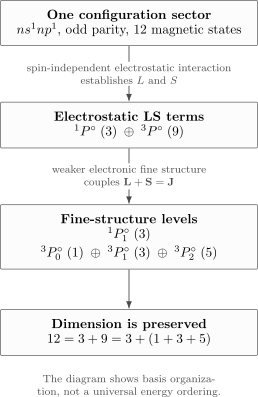
LS coupling organizes a fixed $ns^1np^1$ configuration first into electrostatic $\,{}^1P^\circ$ and $\,{}^3P^\circ$ terms and then into fine-structure $J$ levels. The state count is unchanged at each basis transformation. No universal energy ordering is implied.

Constructing an Atomic LS Basis

The construction proceeds from antisymmetric spin-orbital states, not from distinguishable electrons following separate orbits.

Closed subshells

A completely filled subshell has

$$L_{\mathrm{closed}}=0, \qquad S_{\mathrm{closed}}=0.$$

Its magnetic substates cancel pairwise, and its determinant is a rotational scalar in both orbital and spin space. Closed subshells still contribute to screening, correlation, and the energy, but they do not alter the total $L$ or $S$ obtained by coupling the open subshells.

Coupling subshell parents

Suppose two antisymmetric electron groups have parent terms

$$\alpha_A L_A S_A, \qquad \alpha_B L_B S_B.$$

Their allowed resultants satisfy

$$\begin{aligned} L_{\min}&=|L_A-L_B|,\\ L&=L_{\min},L_{\min}+1,\ldots,L_A+L_B, \end{aligned}$$

and

$$\begin{aligned} S_{\min}&=|S_A-S_B|,\\ S&=S_{\min},S_{\min}+1,\ldots,S_A+S_B. \end{aligned}$$

The labels $\alpha_A$ and $\alpha_B$ retain any ancestry needed to distinguish repeated parent terms. The procedure can be applied recursively to additional open groups.

For nonequivalent groups, every angular-momentum resultant allowed by the triangle rules is normally present. For equivalent electrons in the same $n\ell$ subshell, fermionic antisymmetry removes some formal resultants. For example,

$$p^2 \quad\longrightarrow\quad {}^1S,\ {}^1D,\ {}^3P,$$

not every term obtainable by naively coupling two $\ell=1$, $s=1/2$ particles. Pauli Principle in Atoms owns the exclusion constraints, and Slater Determinants in Atoms develops the determinant-to-CSF construction.

From orbital and spin projections to J

An orbital-and-spin-adapted CSF may be written

$$|\gamma L M_L;S M_S\rangle.$$

Coupling $\mathbf L$ and $\mathbf S$ gives

$$\begin{aligned} |\gamma LSJM_J\rangle ={}& \sum_{M_L,M_S} \langle LM_L,SM_S|JM_J\rangle \\ &\times |\gamma L M_L;S M_S\rangle. \end{aligned}$$

The Clebsch–Gordan coefficient vanishes unless

$$M_J=M_L+M_S.$$

For fixed $L$ and $S$, the allowed values are

$$J = |L-S|, |L-S|+1, \ldots, L+S.$$

This is a unitary change of basis. It neither changes the Hamiltonian nor adds an approximation.

Dimension closure

An $LS$ term contains

$$(2L+1)(2S+1)$$

orbital-spin projection states. Coupling to $J$ reorganizes them according to

$$\sum_{J=|L-S|}^{L+S}(2J+1) =(2L+1)(2S+1).$$

For a complete configuration space,

$$N_{\mathrm{det}} = \sum_{\gamma,L,S} (2L+1)(2S+1),$$

where repeated terms require distinct $\gamma$ labels. Failure of this count usually signals a missing term, an excluded equivalent-electron restriction, or double counting.

Configurations, Terms, Levels, and States

These words describe different layers:

Layer	Typical notation	What it specifies
configuration	$2p^2$	occupations in a chosen orbital basis
electrostatic term	$2p^2\,{}^3P$	a subspace of definite $L$, $S$, and parity
fine-structure level	$2p^2\,{}^3P_2$	a definite $J$ member of that term
magnetic state	$\lvert\gamma LSJM_J\rangle$	one projection state within a level
physical eigenstate	$\lvert\Psi_{\nu JM_J\pi}\rangle$	an eigenvector, often mixing several basis terms

The standard symbol

$${}^{2S+1}L_J$$

records multiplicity, total orbital angular momentum, and total electronic angular momentum. Odd parity is conventionally marked by a superscript degree symbol. The label $\gamma$ is usually omitted from a short spectroscopic name but may encode configuration, parent term, seniority, or an ordinal prefix such as $a$, $b$, or $z$.

A term symbol is not a wavefunction. Two different CSFs can share $L$, $S$, $J$, and parity, and a physical level can be a superposition of both.

Fine Structure Within an Isolated Term

The microscopic spin–orbit operator in a multi-electron atom has the approximate one-electron form

$$H_{\mathrm{so}} \sim \sum_i \zeta_i(r_i)\, \mathbf \ell_i\cdot\mathbf s_i,$$

supplemented at the same accuracy goal by other relativistic interactions. It is not generally identical to a constant times $\mathbf L\cdot\mathbf S$ over the full atomic Hilbert space.

When one $LS$ term is well isolated, however, the rotationally invariant fine-structure operator projected into that term often has the leading effective form

$$H_{\mathrm{fs}}^{\mathrm{eff}} = A_{\gamma LS}\, \mathbf L\cdot\mathbf S.$$

Using

$$J^2 = L^2+S^2 +2\mathbf L\cdot\mathbf S,$$

one obtains

$$\begin{aligned} \Delta E_{\gamma LSJ} ={}& \frac{A_{\gamma LS}}{2} \bigl[ J(J+1) -L(L+1) \\ &\qquad -S(S+1) \bigr]. \end{aligned}$$

This formula is an effective first-order result for an isolated term. It is not the general fine-structure Hamiltonian.

The Landé interval rule

Adjacent levels then satisfy

$$E_J-E_{J-1} = A_{\gamma LS}J.$$

Thus the adjacent intervals are proportional to the larger $J$. For a $\,{}^3P$ term with $J=0,1,2$,

$$\frac{E_2-E_1}{E_1-E_0}=2$$

when the effective $\mathbf L\cdot\mathbf S$ model is accurate and the levels are ordered with the same sign of $A_{\gamma LS}$.

The rule is a diagnostic, not a definition of LS coupling. Spin–spin and spin–other-orbit terms, second-order mixing, configuration interaction, and experimental misassignment can all change the intervals. Conversely, an approximately correct interval ratio does not prove that every eigenvector is pure.

The term centroid

Define the statistical-weight centroid

$$\bar E_{\gamma LS} = \frac{ \displaystyle \sum_J(2J+1)E_{\gamma LSJ} }{ (2L+1)(2S+1) }.$$

For the pure $A_{\gamma LS}\mathbf L\cdot\mathbf S$ splitting,

$$\sum_J (2J+1) \Delta E_{\gamma LSJ} =0,$$

so $\bar E_{\gamma LS}$ equals the unsplit term energy to first order. This trace relation is useful when comparing term calculations with resolved experimental levels.

Spectroscopic Diagnostics

No single observable certifies a coupling scheme. A defensible assignment combines eigenvectors, energy patterns, magnetic response, and transition data.

Eigenvector composition

Within a fixed $J^\pi$ sector, write a normalized level as

$$|\Psi_{\nu JM_J\pi}\rangle = \sum_{\gamma,L,S} c_{\gamma LS}^{(\nu J\pi)} |\gamma LSJM_J\pi\rangle,$$

with

$$\sum_{\gamma,L,S} \left| c_{\gamma LS}^{(\nu J\pi)} \right|^2 =1.$$

The largest squared coefficient is often called the purity in that coupling scheme:

$$P_{\mathrm{LS}} = \max_{\gamma,L,S} \left| c_{\gamma LS}^{(\nu J\pi)} \right|^2.$$

This is useful bookkeeping, but it is basis dependent. It changes with the orbital set, configuration space, coupling order, and phase convention. It is not a directly measured probability that the atom “is in a term.”

The NIST Atomic Spectra Database help reports leading eigenvector percentages when evaluated calculations support them and explicitly warns that a leading component need not give a unique or highly pure level name.

The Landé g factor

For a pure $LSJ$ level with $J>0$, the weak-field magnetic factor is

$$\begin{aligned} g_J&=g_LC_L+g_SC_S,\\ C_L&= \frac12+ \frac{L(L+1)-S(S+1)} {2J(J+1)},\\ C_S&= \frac12+ \frac{S(S+1)-L(L+1)} {2J(J+1)}. \end{aligned}$$

Here $g_L\simeq1$ and $g_S\simeq2.002319$. Setting $g_L=1$ and $g_S=2$ gives the familiar Landé formula

$$g_J = \frac32+ \frac{ S(S+1)-L(L+1) }{ 2J(J+1) }.$$

For $J=0$, there is no first-order electronic Zeeman splitting and the formula with a vanishing denominator should not be used.

The agreement of a measured $g$ factor with the LS value is often a sharper assignment test than energy order alone. In a simple mixture whose magnetic moment is diagonal in the chosen LS basis,

$$g_{\nu J} \approx \sum_{\gamma,L,S} \left| c_{\gamma LS}^{(\nu J)} \right|^2 g_{LSJ}.$$

This relationship also shows why a measured intermediate value can reveal mixing.

A hierarchy of checks

A practical assessment asks:

• Do the number and $J$ values of observed levels match one $LS$ term?
• Are adjacent intervals approximately compatible with an isolated-term model?
• Are measured $g$ factors close to the corresponding Landé values?
• Do strong and weak transition branches follow pure-$LS$ expectations?
• Are intercombination lines weak at the scale predicted by the inferred admixture?
• Do calculated leading percentages remain stable as the orbital and configuration spaces are enlarged?
• Does another coupling scheme give a substantially more compact eigenvector description?

Selection Rules in the LS Limit

For an electric-dipole transition between field-free electronic levels, exact rotational and parity constraints give

$$\Delta J=0,\pm1, \qquad J=0\not\leftrightarrow J'=0,$$

and

$$\pi_f=-\pi_i.$$

For a specified polarization component $q$,

$$\Delta M_J=q, \qquad q=0,\pm1.$$

In the nonrelativistic pure-$LS$ limit, the electric-dipole operator does not act on spin, so

$$\Delta S=0.$$

Its rank-one orbital character also gives

$$\Delta L=0,\pm1, \qquad L=0\not\leftrightarrow L'=0.$$

The $J$ and parity rules follow from exact symmetries of the declared field-free Hamiltonian and transition operator. The $\Delta S$ and $\Delta L$ statements depend on the purity of the LS labels. Relativistic and configuration mixing can open an intercombination line without violating the exact $J^\pi$ rules.

Fine-structure line strengths

When the initial and final levels are pure LS states with the same spin $S$, let $D_{J_fJ_i}^{(1)}$ denote the level-reduced dipole matrix element and $D_{L_fL_i}^{(1)}$ the term-reduced orbital matrix element. Angular recoupling gives

$$\begin{aligned} D_{J_fJ_i}^{(1)} ={}& (-1)^{L_f+S+J_i+1} \\ &\times \sqrt{ (2J_f+1)(2J_i+1) } \\ &\times \begin{Bmatrix} L_f & J_f & S\\ J_i & L_i & 1 \end{Bmatrix} D_{L_fL_i}^{(1)}. \end{aligned}$$

The $6j$ symbol distributes one term-to-term reduced matrix element among the allowed fine-structure components. This predicts relative angular strengths only under the stated assumptions; different radial integrals, configuration interaction, and term mixing can modify observed ratios.

How an intercombination line appears

Consider two basis terms with the same $J^\pi$ but different spin:

$$|s\rangle = |\gamma_s\,{}^1P^\circ_1\rangle, \qquad |t\rangle = |\gamma_t\,{}^3P^\circ_1\rangle.$$

Spin-dependent interactions may produce

$$\begin{aligned} |\widetilde s\rangle &= \cos\theta\,|s\rangle -\sin\theta\,|t\rangle, \\ |\widetilde t\rangle &= \sin\theta\,|s\rangle +\cos\theta\,|t\rangle. \end{aligned}$$

If an initial singlet couples strongly to $|s\rangle$ and not to $|t\rangle$ in the LS limit, its transition amplitude to the triplet-like eigenstate is proportional to $\sin\theta$. The corresponding line strength is of order

$$\sin^2\theta$$

relative to a comparable allowed singlet transition. “Spin forbidden” therefore means vanishing in a stated limit, not impossible in the full atom.

Worked Example: Helium 1s2p

For the nonequivalent-electron configuration $1s\,2p$,

$$\ell_{1s}=0, \qquad \ell_{2p}=1,$$

so the only total orbital angular momentum is

$$L=1.$$

Two spins $1/2$ give

$$S=0,\ 1.$$

The electrostatic terms are therefore

$$1s\,2p\;{}^1P^\circ, \qquad 1s\,2p\;{}^3P^\circ.$$

Their fine-structure levels are

$${}^1P^\circ_1$$

and

$${}^3P^\circ_0, \quad {}^3P^\circ_1, \quad {}^3P^\circ_2.$$

The dimension check is

$$\underbrace{2\times6}_{12\ \mathrm{determinants}} = \underbrace{3}_{\,{}^1P^\circ} + \underbrace{(1+3+5)}_{\,{}^3P^\circ}.$$

This spectrum displays the LS hierarchy unusually clearly. The NIST atomic-spectroscopy compendium quotes an electrostatic $\,{}^3P^\circ-{}^1P^\circ$ separation of about $0.254\ \mathrm{eV}$ for He I $1s2p$, while the spread across the $\,{}^3P^\circ_J$ levels is about $1.32\times10^{-4}\ \mathrm{eV}$. The term separation is therefore roughly three orders of magnitude larger than the fine-structure spread.

The numerical hierarchy does not mean fine structure is irrelevant: it resolves three different $J$ levels and permits weak singlet–triplet mixing where exact $J^\pi$ labels coincide.

Worked Example: The p-Squared Configuration

An $np^2$ subshell has six spin-orbitals and two electrons, so

$$N_{\mathrm{det}} = \binom{6}{2} =15.$$

Antisymmetry permits

$${}^1S, \qquad {}^1D, \qquad {}^3P.$$

Their term dimensions are

$$\begin{aligned} \dim({}^1S)&=1,\\ \dim({}^1D)&=5,\\ \dim({}^3P)&=9, \end{aligned} \qquad 1+5+9=15.$$

Coupling to $J$ gives

$${}^1S_0, \qquad {}^1D_2, \qquad {}^3P_{0,1,2}.$$

All have even parity because

$$\pi=(-1)^{1+1}=+1.$$

The configuration label alone does not determine which term lies lowest. That ordering depends on electrostatic integrals, shell occupancy, and corrections to the chosen Hamiltonian. Nor does LS coupling itself supply the ordering rule: it supplies the basis in which the electrostatic and fine-structure patterns are organized.

Worked Example: Two-Term Intermediate Coupling

Within one $J^\pi$ sector, consider two LS basis states with matrix

$$H = \begin{pmatrix} E_a & V\\ V^* & E_b \end{pmatrix}.$$

After choosing a relative phase so that $V$ is real, the magnitude of the mixing angle obeys

$$|\tan(2\theta)| = \frac{2|V|}{|E_a-E_b|}.$$

The exact energies are

$$E_\pm = \frac{E_a+E_b}{2} \pm \sqrt{ \left( \frac{E_a-E_b}{2} \right)^2 +V^2 }.$$

When $|V|\ll|E_a-E_b|$,

$$|\theta| \approx \frac{|V|}{|E_a-E_b|},$$

and the minority LS weight is approximately

$$\sin^2\theta \approx \frac{|V|^2}{|E_a-E_b|^2}.$$

Near an accidental crossing, the denominator shrinks and the labels can exchange character. Tracking a level only by energy order can then misidentify it; eigenvector overlaps, $g$ factors, and transition patterns provide more reliable continuity.

A Reliable Atomic Workflow

For an actual multi-electron calculation or spectrum:

1. Declare the Hamiltonian. State whether the model is nonrelativistic, Breit–Pauli, Dirac–Coulomb, or includes additional radiative, recoil, nuclear, or field terms.
2. Declare the orbital and configuration space. Configuration percentages have meaning only relative to this representation.
3. Build antisymmetric CSFs. Enforce equivalent-electron restrictions before assigning terms.
4. Block by exact symmetry. In a field-free atom this normally means $J$, $M_J$, and parity; $M_J$ need not be retained explicitly in a reduced calculation.
5. Diagonalize the full retained Hamiltonian. Do not infer physical levels from diagonal term energies alone when off-diagonal mixing is comparable.
6. Transform and label. Report leading $LS$ components, but preserve exact $J^\pi$ labels and any required parentage.
7. Check state counts and orthogonality. The determinant, CSF, and eigenstate dimensions must agree within each symmetry sector.
8. Validate spectroscopically. Compare energies, intervals, $g$ factors, lifetimes, branching fractions, and mixing-sensitive lines.
9. Test stability. Enlarge the orbital and configuration spaces and check whether both observables and reported compositions stabilize.

The label is the end of an analysis, not its starting assumption.

Common Mistakes

• Treating LS coupling as an additional force rather than a basis and hierarchy of interactions.
• Saying $L$ and $S$ are exact for the full relativistic atom while using only $J$ and parity to block the Hamiltonian.
• Comparing an overall spin–orbit scale with a generic Coulomb energy instead of checking off-diagonal matrix elements against same-$J^\pi$ term separations.
• Coupling equivalent electrons by triangle rules without enforcing antisymmetry.
• Confusing multiplicity $2S+1$ with the degeneracy $2J+1$ of one level.
• Assuming a configuration determines one term or a term determines one energy ordering.
• Applying the Landé interval rule to a strongly mixed or nonisolated term without qualification.
• Using the Landé $g$ formula at $J=0$.
• Treating $\Delta S=0$ and $\Delta L=0,\pm1$ as exact relativistic selection rules.
• Interpreting a leading LS percentage as a representation-independent measurement probability.
• Calling every light-atom level pure LS or every heavy-atom level pure $jj$.
• Reporting a short term label without the eigenvector composition when two components are comparable.

Exercises

Exercise 1: Nonequivalent s and p electrons

For an $ns^1np^1$ configuration, list the allowed $LS$ terms and all $J$ levels. Determine parity and verify the total state count.

Solution

The orbital momenta are $\ell_s=0$ and $\ell_p=1$, so

$$L=1.$$

Two spins $1/2$ give

$$S=0,\ 1.$$

Because the electrons occupy nonequivalent subshells, both spin resultants occur:

$${}^1P^\circ, \qquad {}^3P^\circ.$$

The parity is odd:

$$\pi=(-1)^{0+1}=-1.$$

The singlet has only $J=1$, while the triplet has $J=0,1,2$:

$${}^1P^\circ_1, \qquad {}^3P^\circ_{0,1,2}.$$

The $s$ subshell supplies two spin-orbitals and the $p$ subshell six, so there are $2\times6=12$ determinants. The term count is

$$3+(1+3+5)=12.$$

Exercise 2: Equivalent p electrons

The allowed terms of $np^2$ are $\,{}^1S$, $\,{}^1D$, and $\,{}^3P$. Show that they exhaust the determinant space and list their fine-structure levels.

Solution

There are six $np$ spin-orbitals, so

$$N_{\mathrm{det}} = \binom{6}{2} =15.$$

The term dimensions are

$$\begin{aligned} (2L+1)(2S+1) &=1 &&\text{for }{}^1S,\\ &=5 &&\text{for }{}^1D,\\ &=9 &&\text{for }{}^3P. \end{aligned}$$

Their sum is $1+5+9=15$. The fine-structure levels are

$${}^1S_0, \qquad {}^1D_2, \qquad {}^3P_0,\ {}^3P_1,\ {}^3P_2.$$

All have even parity. The dimension closure verifies completeness but does not derive why antisymmetry excludes the other naive two-electron resultants.

Exercise 3: A triplet D term

For an isolated $\,{}^3D$ term described by $H_{\mathrm{fs}}^{\mathrm{eff}}=A\mathbf L\cdot\mathbf S$, find the allowed $J$ values, their shifts from the term centroid, and the adjacent intervals. Verify the weighted-centroid sum.

Solution

Here $L=2$ and $S=1$, so

$$J=1,2,3.$$

Because

$$L(L+1)+S(S+1)=6+2=8,$$

the shifts are

$$\begin{aligned} \Delta E_1 &= \frac A2(2-8) =-3A,\\ \Delta E_2 &= \frac A2(6-8) =-A,\\ \Delta E_3 &= \frac A2(12-8) =2A. \end{aligned}$$

Therefore

$$E_2-E_1=2A, \qquad E_3-E_2=3A,$$

as required by the Landé interval rule. With statistical weights $3$, $5$, and $7$,

$$3(-3A)+5(-A)+7(2A)=0.$$

Thus the first-order splitting leaves the weighted centroid unchanged.

Exercise 4: Magnetic diagnostics for a triplet P term

Using $g_L=1$ and $g_S=2$, compute the Landé $g$ factors for the $J=1$ and $J=2$ levels of a $\,{}^3P$ term. What should be said about $J=0$?

Solution

For $\,{}^3P$, $L=S=1$. The compact formula gives

$$g_J = 1+ \frac{ J(J+1)+2-2 }{ 2J(J+1) } = \frac32$$

for both $J=1$ and $J=2$.

For $J=0$, the formula is undefined because its denominator vanishes. The level has no first-order electronic Zeeman splitting proportional to $M_J$, since only $M_J=0$ exists. Quadratic Zeeman shifts and hyperfine effects can still occur.

Exercise 5: Estimate intermediate coupling

Two same-$J^\pi$ basis terms are separated by $\Delta=1000\ \mathrm{cm}^{-1}$ and coupled by a real matrix element $V=100\ \mathrm{cm}^{-1}$. Estimate the minority weight and the level shifts. If only the minority singlet component supplies an E1 amplitude to a triplet-like state, estimate its strength fraction relative to a comparable allowed line.

Solution

The magnitude of the mixing angle satisfies

$$|\tan(2\theta)| = \frac{2V}{\Delta} =0.2.$$

Hence

$$\theta = \frac12\arctan(0.2) \approx0.0987,$$

and

$$\sin^2\theta \approx9.7\times10^{-3}.$$

Taking the unperturbed energies as $0$ and $1000\ \mathrm{cm}^{-1}$,

$$E_\pm = 500 \pm \sqrt{500^2+100^2} \ \mathrm{cm}^{-1}.$$

Numerically,

$$\begin{aligned} E_-&\approx-9.90\ \mathrm{cm}^{-1},\\ E_+&\approx1009.90\ \mathrm{cm}^{-1}. \end{aligned}$$

If all radial and frequency factors are otherwise comparable, the intercombination strength is approximately the singlet weight,

$$9.7\times10^{-3},$$

or about $1\%$ of the corresponding pure allowed strength. Real line ratios also include differing radial matrix elements and transition frequencies.

Exercise 6: Exact and approximate E1 rules

Classify the following statements for a field-free atom: parity must change; $J=0\leftrightarrow J'=0$ is forbidden; $\Delta S=0$; and $\Delta L=0,\pm1$. Which survive strong intermediate coupling?

Solution

For an electric-dipole operator in a rotationally invariant, parity-conserving field-free atom, parity change and the $J$ triangle rule, including the exclusion of $0\leftrightarrow0$, follow from exact transformation properties. They survive intermediate coupling as long as the stated symmetries and E1 operator remain appropriate.

The rules $\Delta S=0$ and $\Delta L=0,\pm1$ use pure nonrelativistic LS labels. They are exact within that limiting basis but need not constrain fully mixed relativistic eigenstates. Mixing can therefore open nominally spin-forbidden or $L$-forbidden lines while preserving exact parity and $J$ constraints.

Exercise 7: Diagnose an assignment

A candidate $\,{}^3D$ multiplet has three levels with $J=1,2,3$. The observed interval ratio is

$$\frac{E_3-E_2}{E_2-E_1}=1.48,$$

compared with the isolated-term value $3/2$. Measured $g$ factors agree with LS values within $2\%$, and a converged calculation gives leading LS weights of $92\%$, $89\%$, and $91\%$. What conclusion is justified?

Solution

The level count, interval ratio, magnetic factors, and calculated compositions all support $\,{}^3D$ as a useful dominant label. The small interval and $g$ deviations indicate corrections to the simplest isolated $A\mathbf L\cdot\mathbf S$ model, while the roughly $10\%$ minority weights show that the states are not pure.

A defensible conclusion is: “The three levels form a predominantly $\,{}^3D$ multiplet in near-LS coupling, with measurable intermediate-coupling corrections.” It would be too strong to claim exact $L$ and $S$, or to infer that every transition strength must follow pure-LS ratios.

Key Takeaways

• LS coupling is a basis choice promoted to a physical approximation when electrostatic term separations dominate same-$J^\pi$ relativistic mixing.
• The nonrelativistic Coulomb Hamiltonian conserves $L$ and $S$; a relativistic field-free Hamiltonian generally conserves only total $J$ and parity among those labels.
• Antisymmetry determines which equivalent-electron terms exist before $\mathbf L$ and $\mathbf S$ are coupled to $\mathbf J$.
• The transformation from determinant projections to $LSJ$ CSFs is unitary and preserves state counts.
• An isolated term with effective $A\mathbf L\cdot\mathbf S$ splitting obeys the Landé interval rule and has an unchanged statistical-weight centroid.
• Eigenvector percentages, Landé $g$ factors, interval patterns, and line strengths are complementary diagnostics.
• $\Delta S=0$ and $\Delta L=0,\pm1$ are pure-LS E1 rules; exact field-free E1 constraints are stated in terms of $J$, parity, and projection.
• Intermediate coupling is not a failure of quantum numbers altogether: $J^\pi$ can remain exact while $L$ and $S$ become mixed.

Cross-Links

• Term Symbol Reference provides the compact LS, jj, molecular, multiplicity, and parity lookup.
• Multi-Electron Atoms
• Helium Atom
• Electron Configurations
• Pauli Principle in Atoms
• Exchange and Correlation
• Hartree–Fock for Atoms
• Slater Determinants in Atoms
• jj Coupling
• Hund’s Rules
• Atomic Term Symbols
• Fine Structure
• Atomic Selection Rules
• Zeeman Effect in Atoms
• Angular Momentum Coupling Schemes
• Coupled and Uncoupled Bases
• Clebsch–Gordan Coefficients
• Recoupling and Wigner Symbols
• Spin–Orbit Coupling
• Wigner–Eckart Theorem
• Applications to Atomic Spectra
• AMO Physics Roadmap

References

1. W. C. Martin and W. L. Wiese, “Atomic Spectroscopy: An Introduction”, in G. W. F. Drake, ed., Atomic, Molecular, and Optical Physics Handbook, AIP Press, 1996; NIST online revision updated 2025.
2. A. Kramida, Yu. Ralchenko, J. Reader, and the NIST ASD Team, NIST Atomic Spectra Database, version 5.12, National Institute of Standards and Technology, 2024, DOI: 10.18434/T4W30F, accessed 2026-07-21.
3. H. N. Russell and F. A. Saunders, “New Regularities in the Spectra of the Alkaline Earths”, The Astrophysical Journal 61, 38–69 (1925).
4. E. U. Condon and G. H. Shortley, The Theory of Atomic Spectra, Cambridge University Press, 1935.
5. R. D. Cowan, The Theory of Atomic Structure and Spectra, University of California Press, 1981.
6. I. I. Sobelman, Atomic Spectra and Radiative Transitions, 2nd ed., Springer, 1992.
7. R. N. Zare, Angular Momentum: Understanding Spatial Aspects in Chemistry and Physics, Wiley, 1988.
8. W. R. Johnson, Atomic Structure Theory: Lectures on Atomic Physics, Springer, 2007.
9. C. J. Foot, Atomic Physics, Oxford University Press, 2005.
10. B. H. Bransden and C. J. Joachain, Physics of Atoms and Molecules, 2nd ed., Pearson, 2003.
11. H. A. Bethe and E. E. Salpeter, Quantum Mechanics of One- and Two-Electron Atoms, Springer, 1957.
12. C. Froese Fischer, T. Brage, and P. Jönsson, Computational Atomic Structure: An MCHF Approach, Institute of Physics Publishing, 1997.