Fine Structure

Fine structure is the relativistic and spin-dependent splitting of electronic atomic levels beyond the leading nonrelativistic Coulomb or central-field spectrum. In hydrogen, its leading one-electron terms are the relativistic kinetic-energy correction, spin–orbit coupling, and the Darwin contact term. Their sum reorganizes the spectrum by total electronic angular momentum $j$.

In many-electron atoms, fine structure also includes relativistic one- and two-electron interactions that split electronic terms into levels of different total $J$. The result depends on screening, configuration interaction, and the appropriate LS, jj, or intermediate coupling scheme.

This page owns the atomic hierarchy, combined hydrogenic result, spectroscopic interpretation, and many-electron boundary. The general angular algebra of $\mathbf L\cdot\mathbf S$ belongs to Spin–Orbit Coupling; crystal-field projection and Bloch-band consequences belong to Spin–Orbit Coupling in Solids; perturbative diagonalization belongs to Degenerate Perturbation Theory; and the full relativistic wave equation is represented here only through links to the Dirac Equation.

What Fine Structure Means

The word structure refers to successively finer resolution of a spectral feature. A useful hierarchy is:

Layer	Principal origin	Typical labels	Included in fine structure?
gross electronic structure	nonrelativistic binding and electron–electron electrostatics	configuration, $n$, term	no; this is the reference spectrum
fine structure	relativity and electronic spin-dependent interactions	$j$ or $J$	yes
Lamb and other radiative shifts	quantum electrodynamics plus recoil and nuclear terms at precision level	often same $j,J$ labels	no in the strict hierarchy
hyperfine structure	nuclear spin and nuclear multipole moments	$F$	no
isotope shifts	nuclear mass and charge distribution	isotope label	no
Zeeman and Stark structure	applied magnetic and electric fields	field-dressed projections	no

Historical and database conventions can group corrections differently. A trustworthy use of “fine-structure interval” states which centroid, isotope, field-free limit, and theoretical contributions are meant.

Fine structure is not merely spin–orbit coupling

Spin–orbit coupling often produces the most visible splitting in a non-$S$ term, but it is only one part of the relativistic correction. For hydrogen, omitting mass–velocity and Darwin terms gives the wrong absolute level shifts and obscures the characteristic dependence on $n$ and $j$.

For an $S$ state, $L=0$ makes the one-electron spin–orbit term vanish, yet mass–velocity and Darwin corrections remain. The absence of a spin–orbit doublet is not the absence of fine structure.

Expansion Parameter and Scale

For a hydrogenic ion of charge $Z$, the characteristic estimates are

$$\frac{v}{c}\sim Z\alpha, \qquad p\sim m_ecZ\alpha,$$

where $\alpha$ is the fine-structure constant. The gross binding scale is

$$E_{\mathrm{gross}} \sim m_ec^2(Z\alpha)^2,$$

while the leading fine-structure scale is

$$E_{\mathrm{fs}} \sim m_ec^2(Z\alpha)^4.$$

Thus

$$\frac{E_{\mathrm{fs}}}{E_{\mathrm{gross}}} \sim (Z\alpha)^2.$$

This power counting explains why fine structure is small in hydrogen and grows rapidly along a hydrogenic sequence. In neutral many-electron atoms, a universal $Z^4$ rule is not reliable because shielding and orbital penetration change the effective field sampled by each electron.

The expansion assumes $Z\alpha\ll1$ and momenta small compared with $m_ec$. Heavy highly charged ions require a nonperturbative relativistic starting point, followed by recoil, finite-nuclear-size, Breit, and radiative corrections appropriate to the desired accuracy.

Effective One-Electron Hamiltonian

Consider a spin-$1/2$ electron in a static central potential energy $V(r)$, with no applied electromagnetic field. The nonrelativistic reference is

$$H_0=\frac{\mathbf p^2}{2m_e}+V(r).$$

Through order $1/c^2$, the leading one-electron fine-structure operator is written

$$H_{\mathrm{fs}}^{(1)} =H_{\mathrm{mv}}+H_{\mathrm{so}}+H_D.$$

This form is obtained from the low-energy expansion of relativistic spinor dynamics, such as a Foldy–Wouthuysen transformation. It is an effective Hamiltonian with a specified order, not three independent fundamental forces.

Relativistic Kinetic-Energy Correction

The exact free-particle kinetic energy is

$$T=\sqrt{m_e^2c^4+p^2c^2}-m_ec^2.$$

Expanding in $p/(m_ec)$ gives

$$T =\frac{p^2}{2m_e} -\frac{p^4}{8m_e^3c^2} +O(c^{-4}).$$

The leading mass–velocity operator is therefore

$$H_{\mathrm{mv}} =-\frac{p^4}{8m_e^3c^2}.$$

Its expectation value is negative: relativistic kinematics makes a bound level more negative relative to the nonrelativistic reference at this order. Because $p^4$ weights high-momentum components strongly, compact and penetrating orbitals are especially sensitive.

The name “mass–velocity” is historical shorthand. One should not replace $m_e$ by a classical speed-dependent mass inside the Schrödinger equation; the operator follows from expanding the relativistic dispersion relation.

Spin–Orbit Term

For a central potential, including the Thomas factor, the leading one-electron operator is

$$H_{\mathrm{so}} =\frac{1}{2m_e^2c^2} \frac{1}{r}\frac{dV}{dr} \mathbf L\cdot\mathbf S.$$

The angular eigenvalue in a state $|\ell,s;j,m_j\rangle$ is

$$\begin{aligned} \langle\mathbf L\cdot\mathbf S\rangle &=\frac{\hbar^2}{2}\Lambda_{\ell s j},\\ \Lambda_{\ell s j} &=j(j+1)-\ell(\ell+1)\\ &\quad-s(s+1). \end{aligned}$$

For an electron, $s=1/2$ and $j=\ell\pm1/2$ when $\ell>0$. Rotational symmetry preserves degeneracy among the $2j+1$ values of $m_j$ while permitting different $j$ multiplets to split.

For a point Coulomb potential,

$$V(r)=-\frac{Ze^2}{4\pi\epsilon_0r},$$

so

$$H_{\mathrm{so}} =\frac{Ze^2}{8\pi\epsilon_0m_e^2c^2r^3} \mathbf L\cdot\mathbf S.$$

The apparent $r^{-3}$ singularity is harmless for the nonzero-$\ell$ hydrogenic expectation values to which this operator applies. For $\ell=0$, $\mathbf L=0$ and the term vanishes. Finite nuclei and relativistic wavefunctions are required when nuclear-region details matter beyond this expansion.

Darwin Term

The Darwin operator is

$$H_D =\frac{\hbar^2}{8m_e^2c^2}\nabla^2V.$$

For a point Coulomb potential, the distributional identity $\nabla^2(1/r)=-4\pi\delta^3(\mathbf r)$ gives

$$H_D =\frac{Ze^2\hbar^2}{8\epsilon_0m_e^2c^2} \delta^3(\mathbf r).$$

Only states with nonzero probability density at the origin receive this point-nucleus contact shift. In the nonrelativistic hydrogenic basis, that means $S$ states. The Darwin term is positive for an attractive point-Coulomb potential and partly offsets the negative mass–velocity shift.

Descriptions in terms of rapid relativistic position fluctuations can provide intuition, but the controlled statement is operator-level: the contact term emerges in the low-energy expansion of the Dirac theory. For a finite nucleus, the delta function is replaced by sensitivity to the nuclear charge distribution.

Hydrogenic Fine Structure

Take an infinitely heavy point nucleus and treat $H_{\mathrm{mv}}$, $H_{\mathrm{so}}$, and $H_D$ consistently through order $(Z\alpha)^4$. Their sum gives

$$\begin{aligned} E_{nj} &=-\frac{m_ec^2(Z\alpha)^2}{2n^2} +\Delta E_{nj}^{\mathrm{fs}},\\ \Delta E_{nj}^{\mathrm{fs}} &=-\frac{m_ec^2(Z\alpha)^4}{2n^4} \left(\frac{n}{j+1/2}-\frac34\right). \end{aligned}$$

The separate terms depend on $\ell$, but their sum depends only on $n$ and $j$ at this order. This is a central structural result, not an accident of notation. It agrees with the expansion of the exact point-Coulomb Dirac energy.

What remains degenerate

Because the energy depends on $j$ rather than separately on $\ell$, states such as

$$nS_{1/2} \quad\text{and}\quad nP_{1/2}$$

remain degenerate in the ideal Dirac–Coulomb problem. Radiative corrections, recoil, and nuclear structure break that degeneracy. The famous $2S_{1/2}$–$2P_{1/2}$ separation is therefore a Lamb-shift question, not a leading fine-structure splitting; Lamb Shift Overview owns that next correction layer.

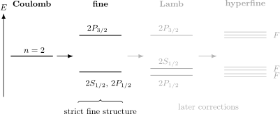
Schematic $n=2$ hierarchy, not to scale. Fine structure separates $2P_{3/2}$ from the ideal Dirac-degenerate $2S_{1/2}$ and $2P_{1/2}$ pair. Radiative and associated corrections produce the Lamb separation, and nuclear spin then produces hyperfine sublevels. The gray columns mark corrections outside the strict fine-structure Hamiltonian.

The n = 2 fine-structure interval

For $Z=1$, the leading difference within the $2P$ term is

$$E_{2P_{3/2}}-E_{2P_{1/2}} =\frac{m_ec^2\alpha^4}{32}.$$

This expression is an infinite-nuclear-mass, leading-order result. Comparison with precision spectroscopy requires reduced-mass and recoil effects, radiative corrections, proton structure, and a careful definition of the measured line centroid.

Many-Electron Fine Structure

The nonrelativistic electronic Hamiltonian for a fixed nucleus is

$$\begin{aligned} H_{\mathrm{NR}} &=\sum_i\left[ \frac{\mathbf p_i^2}{2m_e}+V_{\mathrm{nuc}}(r_i) \right]\\ &\quad+\sum_{i<j} \frac{e^2}{4\pi\epsilon_0r_{ij}}. \end{aligned}$$

Electron–electron repulsion first creates configurations, terms, and correlation structure. Relativistic corrections then act within and between those many-electron states. A schematic Breit–Pauli organization is

$$\begin{aligned} H_{\mathrm{BP}} &=H_{\mathrm{NR}}+H_{1e}^{\mathrm{rel}} +H_{2e}^{\mathrm{rel}},\\ H_{1e}^{\mathrm{rel}} &=\sum_i(H_{\mathrm{mv},i}+H_{D,i}+H_{\mathrm{so},i}),\\ H_{2e}^{\mathrm{rel}} &=H_{\mathrm{oo}}+H_{\mathrm{ss}} +H_{\mathrm{soo}}+\cdots. \end{aligned}$$

Here $H_{\mathrm{oo}}$ denotes orbit–orbit terms, $H_{\mathrm{ss}}$ spin–spin terms, and $H_{\mathrm{soo}}$ spin–other-orbit terms. Authors package contact and mutual spin–orbit contributions differently, so an abbreviation such as “Breit–Pauli” must be accompanied by the actual operator set.

LS coupling

In many light atoms, residual electrostatic interactions organize orbital and spin angular momenta before spin-dependent terms become important:

$$\begin{aligned} \mathbf L&=\sum_i\mathbf l_i,\\ \mathbf S&=\sum_i\mathbf s_i,\\ \mathbf J&=\mathbf L+\mathbf S. \end{aligned}$$

Levels are labeled by term symbols $^{2S+1}L_J$; Atomic Term Symbols owns their configuration, multiplicity, parity, and coupling-scheme grammar. LS Coupling develops the atomic energy-scale criterion, state-count construction, Landé diagnostics, and same-$J^\pi$ mixing that determine whether those labels are physically useful. If the fine-structure operator within one well-isolated term reduces to

$$H_{\mathrm{fs}}^{\mathrm{term}} =A\,\mathbf L\cdot\mathbf S,$$

then

$$\begin{aligned} K_{LSJ} &=J(J+1)-L(L+1)\\ &\quad-S(S+1),\\ E_J &=E_{LS}+\frac{A}{2}K_{LSJ}. \end{aligned}$$

Adjacent intervals obey the Landé interval rule,

$$E_J-E_{J-1}=AJ.$$

This rule is a diagnostic of pure LS coupling, not a universal law. Configuration interaction, spin–spin terms, term mixing, and relativistic radial changes produce deviations.

Term centroid

For the pure $A\mathbf L\cdot\mathbf S$ model, the degeneracy-weighted fine-structure shift averages to zero. Define

$$\overline E_{LS} =\frac{\sum_J(2J+1)E_J} {\sum_J(2J+1)}.$$

Then $\overline E_{LS}=E_{LS}$. This center-of-gravity relation is useful when comparing a relativistically split multiplet with a nonrelativistic term energy. It can fail as a literal identification when fine structure mixes other terms or when the averaging omits levels.

jj and intermediate coupling

In a jj-coupled description, each electron first forms

$$\mathbf j_i=\mathbf l_i+\mathbf s_i,$$

and the $\mathbf j_i$ are combined into total $\mathbf J$. This basis is useful when one-electron spin–orbit splittings compete strongly with residual electrostatic term separations.

jj Coupling develops the relativistic-subshell occupations, equivalent-electron state counts, $9j$ relation to the LS basis, and energy, magnetic, and transition diagnostics needed to test that description.

Most real atoms are not in an exact LS or jj limit. Their eigenstates are mixtures of configuration-state functions with the same conserved total $J$ and parity. “Intermediate coupling” is not a new interaction; it is the need to diagonalize competing electrostatic and relativistic operators without assuming one ideal coupling order.

Level labels then identify dominant components and can exchange character through avoided crossings. A trustworthy table gives mixing coefficients or at least flags ambiguous classifications.

Alkali doublets

An alkali atom has a single valence electron outside a closed shell, so its low-lying $nP$ levels form $P_{1/2}$ and $P_{3/2}$ partners. The principal $D_1$ and $D_2$ lines terminate on those fine-structure levels. Their separation illustrates the trend toward stronger relativistic splitting in heavier atoms, but quantitative values require the actual screened, correlated, and relativistic valence wavefunction. Alkali Atoms owns the optical, hyperfine, cooling, clock, and Rydberg uses of those manifolds.

Connection to the Dirac Equation

For one electron in a static scalar potential, the Dirac Hamiltonian is

$$H_D =c\boldsymbol{\alpha}\cdot\mathbf p +\beta m_ec^2+V(r),$$

where $\boldsymbol{\alpha}$ and $\beta$ are Dirac matrices, not the fine-structure constant. Its four-component spinor combines spin and relativistic kinematics from the start.

For a point Coulomb potential, the bound-state energy depends on $n$ and $j$ through the Dirac angular quantum number. Expanding the positive-energy result in $Z\alpha$ reproduces the combined mass–velocity, spin–orbit, and Darwin shift above. The individual low-energy terms depend on the chosen transformation and order, while their predicted spectrum is the invariant comparison.

Why the Dirac equation is more than a correction formula

A Dirac calculation changes the radial functions as well as the energies. Small components, relativistic contraction of penetrating orbitals, and spinor angular structure affect matrix elements and electron correlation. For heavy atoms, adding a hydrogenic spin–orbit number to a nonrelativistic orbital can miss these coupled changes.

For many electrons, common starting points include Dirac–Hartree–Fock and Dirac–Coulomb configuration-interaction or coupled-cluster methods. The frequency-dependent transverse-photon interaction is approximated at low order by Breit terms. Recoil, finite nuclear size, and QED corrections must then be added without double counting.

A one-particle Dirac equation in a prescribed potential is not the full relativistic interacting theory. Pair creation, vacuum polarization, and radiative self-energy belong to quantum electrodynamics. The reference Dirac Equation records the core formula and conventions; a full relativistic-QM treatment is a separate canonical subject.

Spectroscopic Interpretation

Level interval versus line separation

A fine-structure interval is an energy difference between two atomic levels. A measured spectrum usually contains transition frequencies,

$$h\nu_{ab}=E_a-E_b.$$

The separation of two lines equals an upper-state fine-structure interval only if they share the same lower level and if unresolved hyperfine, isotope, field, and line-shape shifts are handled consistently. Otherwise a difference of transition frequencies combines more than one level interval.

Resolve the hierarchy actually measured

An experimental feature can be:

• unresolved over hyperfine components and reported as an intensity-weighted centroid;
• isotope-specific or a natural-abundance blend;
• shifted by magnetic, electric, blackbody, collisional, or trapping fields;
• broadened by lifetime, Doppler motion, collisions, transit time, or the instrument;
• mixed with a nearby configuration or continuum resonance;
• fitted with a line-shape model whose parameters are correlated.

The quoted “fine-structure splitting” should therefore name the levels, isotope, field extrapolation, centroid convention, and uncertainty model.

Selection rules do not determine splittings

Selection rules say which matrix elements vanish under specified symmetries. They do not calculate the fine-structure energy interval or guarantee that every allowed component is experimentally visible. Transition strengths depend on radial matrix elements, angular coefficients, mixing, populations, polarization, and detection geometry.

Boundaries of the Approximation

Recoil and isotope dependence

Replacing $m_e$ by the reduced mass captures the leading gross-energy recoil, but precision fine structure also contains relativistic recoil and mass-polarization terms. Isotopes differ through both nuclear mass and charge distribution.

Finite nuclear size

Point-nucleus formulas become inadequate for states that penetrate the nucleus or for heavy ions. Finite charge and magnetization distributions modify Dirac orbitals and contact interactions. A fitted nuclear radius carries its own convention and uncertainty.

Radiative corrections

Electron self-energy and vacuum polarization alter the spectrum beyond the Dirac–Coulomb result. They are essential to the Lamb shift and to precision fine-structure theory. Calling every difference between Schrödinger and experiment “the Lamb shift” is as misleading as calling every small splitting “spin–orbit coupling.”

External fields

Fine structure defines a zero-field electronic reference. When Zeeman or Stark energies approach a fine-structure interval, field-dressed states replace the zero-field $J$ labels. In the Paschen–Back regime, coupling orders and approximate quantum numbers change.

Breakdown of low-order power counting

The $1/c^2$ Hamiltonian is controlled only when omitted terms are smaller than the target uncertainty. High $Z$, strong fields, near-degenerate configurations, or nuclear-region observables can invalidate a low-order perturbative treatment even if a numerical correction looks modest.

Validation Workflow

For a defensible fine-structure calculation or comparison:

1. specify the isotope, nuclear model, Hamiltonian, and zero of energy;
2. identify whether the reference is Schrödinger, Pauli/Breit–Pauli, Dirac–Coulomb, or a higher-level effective Hamiltonian;
3. list included one- and two-electron relativistic, recoil, nuclear, and radiative terms;
4. use degenerate or quasi-degenerate diagonalization when states of the same $J$ and parity are close;
5. converge radial grids, basis sets, correlation spaces, and angular cutoffs;
6. compare both absolute term centroids and internal $J$ intervals;
7. test level assignments and mixing against several observables, not energy alone;
8. match experimental centroid, isotope, field, and line-shape conventions;
9. assign an uncertainty to the final interval from omitted physics and numerical convergence.

Agreement for one splitting can result from cancellation between correlation and relativistic errors. Transfer to another term, charge state, or transition amplitude must be tested rather than assumed.

Common Mistakes

• Equating fine structure with spin–orbit coupling alone. Mass–velocity and Darwin terms are required even in one-electron atoms.
• Applying spin–orbit formulas to $S$ states. The $\mathbf L\cdot\mathbf S$ term vanishes for $L=0$, although other relativistic shifts remain.
• Using ordinary functions instead of distributions for the Darwin term. The point-Coulomb Laplacian contains $\delta^3(\mathbf r)$.
• Adding separately derived corrections with inconsistent conventions. The nuclear mass, potential, wavefunctions, and perturbative order must match.
• Calling the $2S_{1/2}$–$2P_{1/2}$ interval fine structure. It vanishes in the ideal Dirac–Coulomb spectrum and is led by the Lamb shift.
• Assuming a universal $Z^4$ law in neutral atoms. Screening and penetration alter radial scaling.
• Treating LS or jj labels as exact in intermediate coupling. They are dominant-component labels unless the limiting hierarchy is controlled.
• Using the Landé interval rule after strong term mixing. The rule assumes a single isolated $A\mathbf L\cdot\mathbf S$ term.
• Comparing a level interval with an arbitrary line separation. Shared endpoints and centroid conventions must be checked.
• Ignoring hyperfine, isotope, and field structure in experimental data. Unresolved components can shift a fitted centroid.
• Treating a one-particle Dirac model as complete QED. Radiative, pair, and transverse-photon physics require a broader framework.

Exercises

1. Relativistic dispersion and power counting

Expand the free relativistic kinetic energy through order $p^4$. Then use $p\sim m_ecZ\alpha$ to show the scale of the first correction relative to the gross kinetic energy.

Solution

Write

$$T=m_ec^2 \left[\sqrt{1+\frac{p^2}{m_e^2c^2}}-1\right].$$

Using $\sqrt{1+x}=1+x/2-x^2/8+O(x^3)$ gives

$$T=\frac{p^2}{2m_e} -\frac{p^4}{8m_e^3c^2} +O(p^6).$$

The gross term scales as

$$\frac{p^2}{2m_e} \sim m_ec^2(Z\alpha)^2,$$

whereas the correction scales as

$$\frac{p^4}{8m_e^3c^2} \sim m_ec^2(Z\alpha)^4.$$

Their ratio is of order $(Z\alpha)^2$, as expected for the leading relativistic correction.

2. Darwin shift and S states

Show that a point-Coulomb Darwin term has zero first-order expectation value in a nonrelativistic hydrogenic state with $\ell>0$. For a hydrogenic $1S$ state, use

$$|\psi_{1S}(0)|^2=\frac{Z^3}{\pi a_0^3}$$

to show that the infinite-mass Darwin shift is

$$\Delta E_D(1S) =\frac12m_ec^2(Z\alpha)^4.$$

Solution

The expectation value of the contact operator is

$$\langle\delta^3(\mathbf r)\rangle =|\psi(0)|^2.$$

Hydrogenic radial wavefunctions behave as $R_{n\ell}(r)\propto r^\ell$ near the origin. Thus $\psi(0)=0$ for $\ell>0$, and their point-nucleus Darwin shift vanishes.

For $1S$,

$$\begin{aligned} \Delta E_D &=\frac{Ze^2\hbar^2}{8\epsilon_0m_e^2c^2} \frac{Z^3}{\pi a_0^3}\\ &=\frac12m_ec^2(Z\alpha)^4, \end{aligned}$$

where $e^2/(4\pi\epsilon_0)=\alpha\hbar c$ and $a_0=\hbar/(m_ec\alpha)$ were used. The positive contact shift is only one contribution; it must be combined with the mass–velocity term to obtain the full $1S$ fine correction.

3. The ³P Landé intervals

For a pure $^3P$ term, $L=1$ and $S=1$. Using $H=A\mathbf L\cdot\mathbf S$, find the shifts for $J=0,1,2$, verify the Landé interval rule, and check the degeneracy-weighted centroid.

Solution

Since $L(L+1)=S(S+1)=2$,

$$\Delta E_J =\frac A2[J(J+1)-4].$$

Therefore

$$\begin{array}{c|ccc} J&0&1&2\\ \hline \Delta E_J&-2A&-A&A \end{array}$$

and

$$E_1-E_0=A, \qquad E_2-E_1=2A.$$

These are $AJ$ for $J=1$ and $2$. With degeneracies $2J+1=1,3,5$,

$$\frac{1(-2A)+3(-A)+5(A)}{1+3+5}=0.$$

The fine-structure shifts leave the term center of gravity unchanged in this ideal model. Significant experimental departures from the $1:2$ interval ratio diagnose additional operators or term mixing.

4. Hydrogen n = 2 splitting

Use the leading hydrogenic fine-structure formula to compute $\Delta E_{2,1/2}^{\mathrm{fs}}$ and $\Delta E_{2,3/2}^{\mathrm{fs}}$. Show that the $2P_{3/2}$–$2P_{1/2}$ interval is $m_ec^2\alpha^4/32$. What does the same formula predict for $2S_{1/2}$ versus $2P_{1/2}$?

Solution

For $n=2$, the common coefficient is $-m_ec^2\alpha^4/32$. For $j=1/2$,

$$\frac{n}{j+1/2}-\frac34 =2-\frac34=\frac54,$$

so

$$\Delta E_{2,1/2}^{\mathrm{fs}} =-\frac{5m_ec^2\alpha^4}{128}.$$

For $j=3/2$,

$$\frac{n}{j+1/2}-\frac34 =1-\frac34=\frac14,$$

giving

$$\Delta E_{2,3/2}^{\mathrm{fs}} =-\frac{m_ec^2\alpha^4}{128}.$$

The difference is

$$E_{2P_{3/2}}-E_{2P_{1/2}} =\frac{m_ec^2\alpha^4}{32}.$$

Both $2S_{1/2}$ and $2P_{1/2}$ have the same $n=2,j=1/2$ in the ideal result, so they remain degenerate. Their observed separation is led by radiative and associated Lamb-shift physics.

5. Classify the correction

Classify each contribution as gross electronic, fine, radiative/Lamb, hyperfine, isotope/recoil, or external-field structure: (a) $-p^4/(8m_e^3c^2)$; (b) $A\mathbf I\cdot\mathbf J$; (c) electron self-energy; (d) $-\mathbf d\cdot\mathbf E$ from an applied field; (e) finite reduced mass; (f) spin–other-orbit interaction.

Solution

Contribution	Classification	Reason
(a) relativistic $p^4$ term	fine structure	leading relativistic electronic kinetic correction
(b) $A\mathbf I\cdot\mathbf J$	hyperfine structure	couples nuclear and electronic angular momenta
(c) electron self-energy	radiative/Lamb	QED loop correction beyond Dirac–Coulomb theory
(d) applied electric field	external-field Stark structure	depends on an imposed field
(e) finite reduced mass	isotope/recoil	depends on nuclear mass; leading kinematic recoil
(f) spin–other-orbit	fine structure	relativistic electronic two-body interaction

The categories organize a calculation but do not make contributions numerically independent. Precision work must use a consistent effective Hamiltonian so recoil, nuclear, Breit, and radiative pieces are not double counted.

Cross-Links

• Common Atomic Hamiltonians gives the compact Pauli correction and shows where it sits in a declared atomic Hamiltonian.
• Atomic Term Symbols explains the labels whose $J$ levels are split by fine structure.
• LS Coupling develops the isolated-term approximation, interval rule, magnetic diagnostics, and intermediate-coupling boundary.
• jj Coupling develops the complementary relativistic-subshell limit and its spectroscopic diagnostics.
• Hydrogen as Atomic Prototype places fine structure in the full experimental correction ladder.
• Lamb Shift Overview explains how QED, recoil, and nuclear terms lift the surviving Dirac degeneracy.
• Zeeman Effect in Atoms explains when a magnetic field preserves $J$ and when the fine-structure Paschen–Back regime replaces it with uncoupled projections.
• Spin–Orbit Coupling is the canonical home for $\mathbf L\cdot\mathbf S$ angular algebra and multiplet counting.
• Angular-Momentum Coupling Schemes compares LS, jj, and intermediate coupling.
• Degenerate Perturbation Theory explains why corrections must be diagonalized inside a degenerate manifold.
• Hydrogen Atom supplies the nonrelativistic Coulomb states used in the leading perturbative calculation.
• Degeneracy of the Hydrogen Atom develops the accidental symmetry that fine structure partially lifts.
• Pauli Equation and Dirac Equation give compact relativistic formula references.
• Sommerfeld Model explains the historically successful but nonmodern orbit picture of hydrogen fine structure.

References

1. H. A. Bethe and E. E. Salpeter, Quantum Mechanics of One- and Two-Electron Atoms (Springer, 1957), Chapters 4–6.
2. J. J. Sakurai and J. Napolitano, Modern Quantum Mechanics, 3rd ed. (Cambridge University Press, 2021), sections on the Dirac equation and nonrelativistic reduction.
3. C. J. Foot, Atomic Physics (Oxford University Press, 2005), Chapters 2–5.
4. B. H. Bransden and C. J. Joachain, Physics of Atoms and Molecules, 2nd ed. (Pearson, 2003), Chapters 5–8.
5. I. P. Grant, Relativistic Quantum Theory of Atoms and Molecules: Theory and Computation (Springer, 2007), doi:10.1007/978-0-387-35069-1.
6. W. R. Johnson, Atomic Structure Theory: Lectures on Atomic Physics (Springer, 2007), doi:10.1007/978-3-540-68013-0.
7. E. U. Condon and G. H. Shortley, The Theory of Atomic Spectra (Cambridge University Press, 1935), Chapters 6–12.
8. L. L. Foldy and S. A. Wouthuysen, “On the Dirac Theory of Spin 1/2 Particles and Its Non-Relativistic Limit,” Physical Review 78, 29–36 (1950), doi:10.1103/PhysRev.78.29.
9. G. Breit, “The Effect of Retardation on the Interaction of Two Electrons,” Physical Review 34, 553–573 (1929), doi:10.1103/PhysRev.34.553.
10. H. A. Bethe, “The Electromagnetic Shift of Energy Levels,” Physical Review 72, 339–341 (1947), doi:10.1103/PhysRev.72.339.
11. M. I. Eides, H. Grotch, and V. A. Shelyuto, “Theory of Light Hydrogenlike Atoms,” Physics Reports 342, 63–261 (2001), doi:10.1016/S0370-1573(00)00077-6.
12. A. Kramida, Y. Ralchenko, J. Reader, and the NIST ASD Team, NIST Atomic Spectra Database, National Institute of Standards and Technology, doi:10.18434/T4W30F.