Hyperfine Structure

Hyperfine structure is the splitting and mixing of atomic levels caused by electromagnetic interactions between the nucleus and the electrons. The leading terms couple the nuclear magnetic dipole moment and electric quadrupole moment to electronic fields at the nucleus. They resolve a fine-structure level of electronic angular momentum $J$ into levels labeled by the total atomic angular momentum

$$\mathbf F=\mathbf I+\mathbf J,$$

where $I$ is the nuclear spin.

The word hyperfine denotes a layer of structure finer than electronic fine structure. It is not another name for spin–orbit coupling: fine structure couples electronic degrees of freedom and is present even for a spinless nucleus, while hyperfine structure depends on the isotope’s nuclear spin and electromagnetic moments.

This page is the canonical home for the atomic hyperfine Hamiltonian, its $F$-dependent spectrum, hydrogen and alkali examples, and microwave clock transitions. Total Angular Momentum owns the general addition rules, Magnetic Moments and g-Factors owns moment conventions, and Alkali Atoms owns platform-specific optical and cooling applications.

What Hyperfine Structure Resolves

For an isolated atom at successively finer resolution, a useful hierarchy is

$$\begin{gathered} \text{electronic configuration} \\ \downarrow \\ \text{fine-structure level }J \\ \downarrow \\ \text{hyperfine level }F \\ \downarrow \\ \text{Zeeman sublevel }m_F. \end{gathered}$$

The hyperfine interaction is usually much smaller than the electronic separation between different fine-structure levels. Under that hierarchy, one first fixes the electronic state $|\gamma J\rangle$, where $\gamma$ collects configuration and other labels, and then diagonalizes the interaction with nuclear spin inside that $J$ manifold.

Layer	Main degrees of freedom	Typical label	Depends on isotope?
gross electronic structure	orbital motion and electron–electron electrostatics	configuration, term	through mass and field shifts
fine structure	electronic relativity and spin-dependent interactions	$J$	weakly, beyond the ideal electronic model
hyperfine structure	nuclear moments coupled to electronic fields	$F$	yes, strongly
Zeeman structure	atomic moments coupled to an external magnetic field	$m_F$ or uncoupled projections	yes

Two cautions follow. First, an observed optical line may contain several unresolved hyperfine components, so a fitted “line center” need not equal the fine-structure centroid. Second, if hyperfine coupling is not small compared with neighboring electronic intervals, it can mix different $J$ levels and the fixed-$J$ formulas below become only first-order approximations.

Nuclear Spin and Electromagnetic Moments

The nucleus has angular momentum operators

$$\begin{aligned} I^2|I m_I\rangle &= \hbar^2I(I+1)|I m_I\rangle, \\ I_z|I m_I\rangle &= \hbar m_I|I m_I\rangle. \end{aligned}$$

Its magnetic dipole moment is conventionally written

$$\boldsymbol\mu_I = g_I\mu_N\frac{\mathbf I}{\hbar}, \qquad \mu_N = \frac{e\hbar}{2m_p},$$

where $g_I$ is the nuclear $g$ factor and $\mu_N$ is the nuclear magneton. Nuclear magnetic moments are typically smaller than electronic moments because $\mu_N/\mu_B=m_e/m_p$.

The magnetic moment need not be parallel to $\mathbf I$ with a positive coefficient; the sign is carried by $g_I$. Isotopes of the same element can have different $I$, $g_I$, and quadrupole moment, so their hyperfine spectra can differ even when their electronic configurations are nearly identical.

Electric quadrupole moment

A nucleus with $I\ge1$ may possess a nonspherical electric charge distribution characterized by a spectroscopic quadrupole moment $Q$. A spin-$0$ or spin-$1/2$ nucleus cannot carry a permanent rank-2 moment in a stationary angular-momentum eigenstate.

The measured electric-quadrupole hyperfine constant is not $Q$ alone. It is proportional to the product of the nuclear quadrupole moment and the electronic electric-field gradient at the nucleus. Extracting one from the other requires either independent nuclear information or an atomic-structure calculation.

Higher nuclear multipoles, such as a magnetic octupole moment, can produce still smaller terms. They matter in selected precision studies but are outside the standard $A$–$B$ model developed here.

Coupling I and J

Because $\mathbf I$ and $\mathbf J$ act on nuclear and electronic factors, the uncoupled basis is

$$|I m_I\rangle\otimes|\gamma J m_J\rangle.$$

For a rotationally invariant zero-field hyperfine Hamiltonian, the coupled basis is more useful:

$$|\gamma;I J;F m_F\rangle,$$

with

$$F=|I-J|,|I-J|+1,\ldots,I+J$$

and

$$m_F=-F,-F+1,\ldots,F.$$

The state transformation is a Clebsch–Gordan expansion,

$$\begin{aligned} |I J;F m_F\rangle &= \sum_{m_I,m_J} C^{F m_F}_{I m_I,J m_J} \\ &\quad\times |I m_I\rangle |J m_J\rangle. \end{aligned}$$

The dimensions agree:

$$(2I+1)(2J+1) = \sum_{F=|I-J|}^{I+J}(2F+1).$$

At zero external field, rotational symmetry makes all $2F+1$ values of $m_F$ degenerate. Hyperfine coupling correlates nuclear and electronic projections; it does not in general preserve $m_I$ and $m_J$ separately.

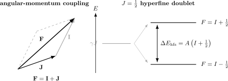
Hyperfine coupling combines $\mathbf I$ and $\mathbf J$ into $\mathbf F$. For an isolated $J=1/2$ level with magnetic-dipole coupling, the two allowed manifolds are $F=I\pm1/2$, separated by $\Delta E_{\mathrm{hfs}}=A(I+1/2)$. The diagram is schematic and not to scale.

Magnetic-Dipole Hyperfine Interaction

Inside an isolated fine-structure level, rotational symmetry makes the leading magnetic-dipole interaction a scalar. With $A$ defined as an energy,

$$H_{\mathrm{M1}} = \frac{A}{\hbar^2} \mathbf I\cdot\mathbf J.$$

The angular identity

$$2\mathbf I\cdot\mathbf J = F^2-I^2-J^2$$

immediately gives

$$E_F^{\mathrm{M1}} = \frac{A}{2}K,$$

where

$$K \equiv F(F+1)-I(I+1)-J(J+1).$$

The constant $A$ includes the nuclear magnetic moment and the electronic magnetic field at the nucleus for the chosen state. It may be positive or negative. The formula predicts angular dependence after $A$ is known; it does not calculate $A$ from first principles.

Hyperfine interval rule

For adjacent $F$ manifolds in the pure magnetic-dipole model,

$$\begin{aligned} E_F-E_{F-1} &= \frac{A}{2} \left[K_F-K_{F-1}\right], \\ &=AF. \end{aligned}$$

Thus adjacent intervals are proportional to the larger $F$. Electric-quadrupole terms, higher multipoles, second-order mixing, and external fields violate this simple interval rule.

The degeneracy-weighted magnetic-dipole centroid is unchanged:

$$\sum_F(2F+1)E_F^{\mathrm{M1}}=0.$$

This trace statement is useful when reconstructing a fine-structure centroid from resolved hyperfine levels. An unweighted average is generally wrong.

Microscopic magnetic contributions

The effective constant $A$ can contain several electronic interactions:

Contribution	Electronic structure	Typical importance
orbital magnetic field	electron orbital current coupled to $\boldsymbol\mu_I$	states with nonzero orbital angular momentum
spin-dipolar field	anisotropic dipole–dipole coupling of electron and nucleus	non-$S$ density and open shells
Fermi contact term	electron spin density at the nucleus	dominant for many $S$ states
relativistic and correlation terms	small components, core polarization, configuration mixing	essential in heavy and many-electron atoms

For a one-electron $S$ state, the leading contact interaction can be written

$$H_{\mathrm F} = \frac{2\mu_0}{3} g_e\mu_Bg_I\mu_N \delta^3(\mathbf r) \frac{\mathbf I\cdot\mathbf S}{\hbar^2},$$

where $g_e$ denotes the positive magnitude convention for the electron spin $g$ factor. Its first-order constant is proportional to

$$A_{nS}^{(0)} \propto g_I\mu_N g_e\mu_B |\psi_{nS}(0)|^2.$$

This explains the strong contact sensitivity of hydrogenic and alkali $S$ states. It does not justify inserting a hydrogenic wavefunction into a heavy neutral atom. Core polarization, exchange, relativistic penetration, finite magnetization, and electronic correlation alter the spin density at the nucleus.

Electric-Quadrupole Hyperfine Interaction

The electric-quadrupole interaction couples rank-2 nuclear and electronic tensors. Schematically,

$$H_{\mathrm{E2}} = \sum_{q=-2}^{2} (-1)^q T_q^{(2)}(\mathrm{nuc}) T_{-q}^{(2)}(\mathrm{el}).$$

Within an isolated $I,J$ manifold, the conventional first-order energy is

$$\begin{aligned} E_F^{\mathrm{E2}} &= B\frac{N_{IJF}}{D_{IJ}}, \\ N_{IJF} &= \frac34K(K+1) -I(I+1)J(J+1), \\ D_{IJ} &= 2I(2I-1)J(2J-1). \end{aligned}$$

The $B$ term exists only when both angular momenta can support the required rank-2 coupling:

$$I\ge1, \qquad J\ge1.$$

For $J=1/2$, the electronic quadrupole expectation vanishes, even if the nucleus has $I\ge1$. This is why alkali $nS_{1/2}$ and $nP_{1/2}$ levels have no first-order electric-quadrupole $B$ term, whereas $nP_{3/2}$ levels can.

The standard dipole-plus-quadrupole model is therefore

$$E_F^{\mathrm{hfs}} = \frac{A}{2}K +E_F^{\mathrm{E2}}.$$

Different databases may tabulate $A$ and $B$ in frequency units, writing $A/h$ and $B/h$ implicitly. Always inspect the convention before substituting a number into an energy formula.

Hydrogen Ground-State Hyperfine Splitting

The hydrogen $1S_{1/2}$ ground state has

$$I=\frac12, \qquad J=\frac12,$$

so the allowed total angular momenta are $F=0$ and $F=1$. For the pure dipole Hamiltonian,

$$\begin{aligned} E_{F=1} &=\frac{A}{4}, \\ E_{F=0} &=-\frac{3A}{4}. \end{aligned}$$

Their difference is

$$\Delta E_{1S}^{\mathrm{hfs}}=A.$$

For ordinary hydrogen, $A>0$, so the $F=1$ triplet lies above the $F=0$ singlet. The evaluated transition frequency quoted by NIST is

$$\nu_{21} = 1420.405\,751\,766\,7(10) \ \mathrm{MHz}.$$

Using $\lambda=c/\nu$ gives approximately

$$\lambda_{21}\simeq21.106\ \mathrm{cm},$$

the celebrated 21 cm line. It is a weak magnetic-dipole transition, but the vast amount of neutral hydrogen in astrophysical environments makes it an exceptionally important probe.

Beyond the Fermi result

The contact model gives the leading scale, not the final prediction. Precision hydrogen theory includes:

• the electron anomalous magnetic moment and other QED corrections;
• relativistic and recoil terms;
• finite proton magnetization and charge distributions;
• the Zemach correction, which couples charge and magnetic form factors;
• proton polarizability and other two-photon-exchange effects;
• weak and hadronic vacuum-polarization contributions at much smaller scales.

The measured interval is extraordinarily precise, while theoretical interpretation is limited more strongly by proton structure. Hyperfine spectroscopy therefore probes a different nuclear combination from the Lamb shift: the Lamb shift is primarily sensitive to charge-radius effects, whereas hyperfine structure is especially sensitive to magnetic structure and spin-dependent two-photon exchange.

The words singlet and triplet describe the coupling of electron and proton spins here. The particles are distinguishable, so this terminology does not impose the exchange-symmetry constraints that apply to two identical electrons.

Alkali Ground-State Doublets

An alkali ground state is approximately $nS_{1/2}$, so $J=1/2$. If $I\ne0$, it splits into

$$F_-=I-\frac12, \qquad F_+=I+\frac12.$$

The dipole energies are

$$\begin{aligned} E_{F_+} &=\frac{AI}{2}, \\ E_{F_-} &=-\frac{A(I+1)}{2}, \end{aligned}$$

so the ground-state interval is

$$\Delta E_{\mathrm{hfs}} = A\left(I+\frac12\right).$$

Representative microwave scales are:

Isotope and state	Nuclear spin	Hyperfine levels	Ground interval
$^1$H $1S_{1/2}$	$1/2$	$F=0,1$	$1.4204057517667\ \mathrm{GHz}$
$^{85}$Rb $5S_{1/2}$	$5/2$	$F=2,3$	about $3.036\ \mathrm{GHz}$
$^{87}$Rb $5S_{1/2}$	$3/2$	$F=1,2$	about $6.835\ \mathrm{GHz}$
$^{133}$Cs $6S_{1/2}$	$7/2$	$F=3,4$	exactly $9.192631770\ \mathrm{GHz}$ as an SI defining frequency

The rubidium entries are rounded orientation values. Precision work should use isotope- and state-specific evaluated constants with uncertainties and source histories, such as the NIST Atomic Spectra Database or the alkali data reviews cited below.

Excited alkali levels

For $nP_{1/2}$, $J=1/2$ again eliminates the first-order $B$ term. For $nP_{3/2}$, $J=3/2$ permits electric-quadrupole structure when $I\ge1$. Optical $D$ lines therefore split into multiple $F\to F'$ components with isotope-dependent spacings and line strengths.

The contact interaction is no longer the entire story in excited or non-$S$ states. Orbital, spin-dipolar, relativistic, and many-body contributions can dominate. Hyperfine constants are stringent tests of electronic wavefunctions near the nucleus and of core-polarization calculations.

Hyperfine anomalies

If $A$ were exactly proportional to the tabulated nuclear magnetic moment, ratios of $A$ between isotopes would follow ratios of nuclear $g$ factors. Finite nuclear magnetization and charge distributions produce small departures known as hyperfine anomalies. They are physical isotope-dependent corrections, not necessarily inconsistent measurements.

Hyperfine Transitions

Within one electronic state, transitions between hyperfine manifolds are typically driven by microwave magnetic fields. In the weak-field coupled basis, the leading magnetic-dipole rules are

$$\Delta F=0,\pm1, \qquad F=0\not\leftrightarrow F'=0,$$

with

$$\Delta m_F=0,\pm1$$

selected by the microwave polarization relative to the quantization axis. These are angular selection rules, not guarantees of equal line strength.

For optical electric-dipole transitions between hyperfine-resolved electronic levels, the same $F$ and $m_F$ rules appear after the electronic reduced matrix element is recoupled to nuclear spin. Atomic Selection Rules gives the operational $6j$ recoupling and polarization rules; their general derivation belongs to the Wigner–Eckart Theorem and Selection Rules pages.

Hyperfine transitions can be exceptionally narrow because the two states share the same electronic configuration and the transition is not an allowed optical electric-dipole decay. Narrowness alone does not make a transition an ideal clock: it must also be preparable, interrogable, reproducible, and insensitive to environmental perturbations.

Hyperfine Transitions in Clocks

For $^{133}$Cs, $I=7/2$ and the $6S_{1/2}$ ground state has $F=3$ and $F=4$. The microwave clock transition uses the states

$$|F=3,m_F=0\rangle \longleftrightarrow |F=4,m_F=0\rangle.$$

At weak magnetic field, a hyperfine Zeeman sublevel has the leading shift

$$\Delta E_Z^{(1)} \simeq g_F\mu_Bm_FB.$$

Each clock state has $m_F=0$, so its diagonal first-order shift vanishes. This makes the transition first-order insensitive near zero field. It is not magnetically insensitive to all orders: the field mixes the two $m_F=0$ hyperfine states and produces a quadratic Zeeman shift.

The SI second

The SI second is defined by fixing the numerical value of the unperturbed $^{133}$Cs ground-state hyperfine transition frequency:

$$\Delta\nu_{\mathrm{Cs}} = 9\,192\,631\,770\ \mathrm{Hz}$$

exactly. The word unperturbed is crucial. A laboratory clock measures atoms in finite fields, at finite temperature, with collisions, motion, microwave interrogation, and gravitational potential. A primary frequency standard evaluates and corrects its realization toward the defining ideal.

Important systematic effects include:

• quadratic Zeeman shifts from the bias magnetic field;
• blackbody-radiation Stark shifts;
• cold-collision and density shifts;
• cavity phase and microwave leakage effects;
• distributed-field and trajectory-dependent Doppler effects;
• imperfect state preparation and residual population in other $m_F$ states;
• gravitational redshift when comparing clocks at different geopotential.

Optical clocks use electronic transitions at much higher frequencies and are not simply “better hyperfine clocks.” Hyperfine averaging and nuclear spin may still matter in their level structure, but their clock transition and systematic ledger belong to a separate precision-metrology treatment.

Magnetic-Field Regimes

The coupled labels $F,m_F$ are reliable when the Zeeman interaction is weak compared with the hyperfine interval. A practical comparison is

$$g_J\mu_BB \ll \Delta E_{\mathrm{hfs}}.$$

In an intermediate field, states with the same conserved $m_F=m_I+m_J$ mix. One should diagonalize

$$H = H_{\mathrm{hfs}} -\boldsymbol\mu_J\cdot\mathbf B -\boldsymbol\mu_I\cdot\mathbf B$$

in fixed-$m_F$ blocks. In the strong-field hyperfine Paschen–Back regime, the uncoupled labels $m_I,m_J$ become more useful. Zeeman Effect in Atoms owns the full Breit–Rabi crossover and polarization-resolved atomic spectra; Zeeman Effect as a Perturbation Example develops the general perturbative field logic.

Avoid assigning a single field-independent $g_F$ through this crossover. The eigenvectors change with $B$, and avoided crossings occur between states with the same exact symmetries.

Experimental Interpretation

Constants are fitted, not read from one arbitrary gap

For a $J=1/2$ doublet, the interval directly determines $A$. For $J\ge1$, several $F$ levels may contain both $A$ and $B$ contributions. Adjacent gaps are then not equal to $A$, and a fit should use the complete level formula with correlated uncertainties.

The fine-structure centroid should be reconstructed with degeneracy weights and a stated convention. If only selected optical transitions are observed, the fit must account for shared upper and lower levels rather than treating line positions as independent level energies.

A spectral peak is apparatus dependent

A hyperfine resonance can be shifted or distorted by magnetic-field gradients, AC Stark shifts, microwave power, optical pumping, collisions, motion, unresolved Zeeman components, and the line-shape model. Reported constants should identify the isotope, electronic state, field extrapolation, frequency reference, and uncertainty budget.

First-order formulas have a domain

The $A$–$B$ expression assumes an isolated electronic $J$ manifold and first-order hyperfine perturbation theory. Nearby electronic levels can be mixed by off-diagonal hyperfine matrix elements, shifting the apparent constants at second order. Precision comparisons must state whether such corrections have been removed, fitted, or included in an effective constant.

Common Mistakes

• Calling hyperfine structure electronic spin–orbit coupling. Hyperfine structure couples nuclear moments to electronic fields; its isotope dependence is essential.
• Writing $\mathbf F=\mathbf I+\mathbf J$ as a numerical equation. It is an operator relation; allowed $F$ values follow angular-momentum addition.
• Assuming $m_I$ and $m_J$ remain good at zero field. The scalar coupling is diagonal in $F,m_F$, not generally in separate projections.
• Using an electron Bohr magneton for the nuclear moment. Nuclear moments are naturally measured in $\mu_N$, though anomalous nuclear $g$ factors can be sizable.
• Including a quadrupole $B$ term for $I=1/2$ or $J=1/2$. A rank-2 diagonal moment is then forbidden.
• Equating every adjacent interval with $A$. The pure dipole rule is $E_F-E_{F-1}=AF$, and a quadrupole term changes it.
• Averaging hyperfine levels without degeneracy weights. That shifts the inferred electronic centroid.
• Treating $A$ as a purely nuclear property. It combines a nuclear moment with an electronic field or spin density.
• Calling $m_F=0$ clock states field independent. Their first-order Zeeman shift vanishes near zero field, but quadratic shifts remain.
• Using zero-field $F$ labels deep in the Paschen–Back regime. The appropriate basis evolves toward $|m_I,m_J\rangle$.
• Reading all digits in a database as universal. State, isotope, unit convention, field condition, and provenance must match the calculation.

Exercises

1. Count the coupled states

For $I=3/2$ and $J=1$, list the allowed values of $F$ and verify that the total number of coupled states equals the uncoupled Hilbert-space dimension.

Solution

Angular-momentum addition gives

$$F=\frac12,\frac32,\frac52.$$

The coupled multiplet dimensions are

$$\begin{aligned} \sum_F(2F+1) &=2+4+6, \\ &=12. \end{aligned}$$

The uncoupled product has dimension

$$(2I+1)(2J+1) = 4\times3 =12.$$

The agreement confirms that coupling reorganizes the same state space; it does not add or remove states.

2. Derive the J = 1/2 doublet

For general nuclear spin $I\ge1/2$ and $J=1/2$, use $E_F=AK/2$ to derive the two energies, their separation, and their degeneracy-weighted centroid.

Solution

For $F_+=I+1/2$,

$$K_+=I, \qquad E_+=\frac{AI}{2}.$$

For $F_-=I-1/2$,

$$K_-=-(I+1), \qquad E_-=-\frac{A(I+1)}{2}.$$

Therefore

$$E_+-E_- = A\left(I+\frac12\right).$$

The degeneracies are $2I+2$ and $2I$. Their weighted sum is

$$\begin{aligned} (2I+2)E_+ &+(2I)E_- \\ &=AI(I+1)-AI(I+1), \\ &=0. \end{aligned}$$

Thus the pure dipole interaction splits the level about its degeneracy-weighted electronic centroid.

3. Diagnose a quadrupole term

Decide whether a first-order electric-quadrupole hyperfine constant $B$ can occur for each pair: (a) $I=1/2,J=3/2$; (b) $I=3/2,J=1/2$; (c) $I=3/2,J=3/2$; (d) $I=0,J=2$. Explain each answer without evaluating the energy formula.

Solution

A diagonal rank-2 coupling requires both $I\ge1$ and $J\ge1$.

Case	$B$ term?	Reason
(a)	no	the spin-$1/2$ nucleus has no permanent quadrupole moment
(b)	no	a $J=1/2$ electronic manifold cannot support the required rank-2 expectation
(c)	yes	both angular momenta are at least one
(d)	no	an $I=0$ nucleus has neither magnetic-dipole nor electric-quadrupole orientation

Hyperfine mixing with other $J$ levels can produce higher-order effects even when a first-order diagonal $B$ constant vanishes, but that does not change this selection rule.

4. Recover the 21 cm wavelength

Using $c=2.99792458\times10^8\ \mathrm{m\,s^{-1}}$ and $\nu=1.4204057518\times10^9\ \mathrm{s^{-1}}$, compute the vacuum wavelength of the hydrogen ground-state hyperfine transition.

Solution

The wavelength is

$$\begin{aligned} \lambda &=\frac{c}{\nu}, \\ &\simeq \frac{2.99792458\times10^8} {1.4204057518\times10^9} \ \mathrm m, \\ &\simeq0.21106\ \mathrm m. \end{aligned}$$

Thus

$$\lambda\simeq21.106\ \mathrm{cm}.$$

The nickname “21 cm line” is a rounded wavelength label; precision work uses the transition frequency and its stated convention.

5. Why clock states still need a bias field

The caesium clock transition uses $m_F=0$ states, for which the first-order Zeeman formula vanishes. Why is a small bias magnetic field still useful, and why must its magnitude be measured?

Solution

A bias field defines a quantization axis and separates the $m_F\ne0$ Zeeman components. That makes state preparation, polarization control, and identification of the clock resonance more robust.

The field cannot be ignored because it mixes the two $m_F=0$ hyperfine states and produces a quadratic Zeeman shift. Spatial inhomogeneity also makes different atomic trajectories sample different shifts. A primary standard therefore measures the field, often using field-sensitive Zeeman transitions, and corrects the clock frequency to the unperturbed limit with an uncertainty.

Cross-Links

• Common Atomic Hamiltonians places the effective $A$–$B$ model beside Zeeman, fine-structure, and Coulomb terms.
• Atomic Selection Rules
• Hydrogen as Atomic Prototype locates hyperfine structure in the complete hydrogen correction hierarchy.
• Alkali Atoms applies ground and excited hyperfine manifolds to $D$ lines, cooling, repumping, clocks, and qubits.
• Fine Structure explains the electronic $J$ levels that hyperfine coupling subsequently resolves.
• Lamb Shift Overview contrasts radiative level shifts with nuclear-spin-dependent structure.
• Total Angular Momentum and Coupled and Uncoupled Bases supply the general $I+J$ algebra.
• Magnetic Moments and g-Factors defines $g$ factors, Bohr and nuclear magnetons, and sign conventions.
• Wigner–Eckart Theorem provides the tensor reduction underlying dipole and quadrupole matrix elements.
• Zeeman Effect in Atoms gives the Breit–Rabi spectrum, Paschen–Back regime map, and polarization-resolved line interpretation.
• Precision Spectroscopy carries the caesium transition into frequency realization, systematic-shift budgets, optical comparisons, and tests of constants.
• Atomic Clocks places the caesium and other hyperfine transitions inside beam, vapor-cell, maser, and fountain clock architectures.
• Zeeman Effect as a Perturbation Example gives the general field-splitting framework.
• Atomic Spectra Experiment Entry gives broader guidance on line assignments and evaluated data.

References

1. C. J. Foot, Atomic Physics (Oxford University Press, 2005), Chapters 2, 6, and 7.
2. G. K. Woodgate, Elementary Atomic Structure, 2nd ed. (Oxford University Press, 1980), Chapters 9–12.
3. I. I. Sobelman, Atomic Spectra and Radiative Transitions, 2nd ed. (Springer, 1992), doi:10.1007/978-3-642-76907-8.
4. E. Fermi, “Über die magnetischen Momente der Atomkerne,” Zeitschrift für Physik 60, 320–333 (1930), doi:10.1007/BF01339933.
5. G. Breit and I. I. Rabi, “Measurement of Nuclear Spin,” Physical Review 38, 2082–2083 (1931), doi:10.1103/PhysRev.38.2082.2.
6. E. Arimondo, M. Inguscio, and P. Violino, “Experimental Determinations of the Hyperfine Structure in the Alkali Atoms,” Reviews of Modern Physics 49, 31–75 (1977), doi:10.1103/RevModPhys.49.31.
7. M. Allegrini, E. Arimondo, and L. A. Orozco, “Survey of Hyperfine Structure Measurements in Alkali Atoms,” Journal of Physical and Chemical Reference Data 51, 043102 (2022), doi:10.1063/5.0098061.
8. National Institute of Standards and Technology, Atomic Spectroscopy: Atomic States, Shells, and Configurations, including the evaluated $^1$H ground-state hyperfine interval.
9. A. Kramida, Y. Ralchenko, J. Reader, and the NIST ASD Team, NIST Atomic Spectra Database, National Institute of Standards and Technology, doi:10.18434/T4W30F.
10. D. A. Steck, Alkali D Line Data, isotope-resolved reference sheets with constants, conventions, and source histories.
11. Bureau International des Poids et Mesures, SI Base Unit: Second, defining $\Delta\nu_{\mathrm{Cs}}=9\,192\,631\,770\ \mathrm{Hz}$ exactly.
12. C. E. Carlson, V. Nazaryan, and K. Griffioen, “Proton Structure Corrections to Electronic and Muonic Hydrogen Hyperfine Splitting,” Physical Review A 78, 022517 (2008), doi:10.1103/PhysRevA.78.022517.