Lamb Shift Overview

The Lamb shift is the difference between an atomic energy level and the value predicted by an idealized relativistic Coulomb model, or, in its most famous usage, the measured separation between hydrogen’s $2S_{1/2}$ and $2P_{1/2}$ levels. Those two levels are degenerate in the point-nucleus Dirac–Coulomb problem. In real hydrogen, the $2S_{1/2}$ level lies higher.

That discrepancy is small on an atomic scale and conceptually decisive. It cannot be produced by merely solving the nonrelativistic Schrödinger equation more accurately, and it is not part of leading fine structure. Its dominant origin is the interaction of the bound electron with the quantized electromagnetic field. Electron self-energy, vacuum polarization, recoil, radiative-recoil terms, and nuclear structure must be combined consistently before theory can be compared with a precision measurement.

This page owns the atomic interpretation, correction hierarchy, experimental logic, and handoff to quantum electrodynamics. It does not derive renormalized bound-state QED from Feynman diagrams. Fine Structure supplies the Dirac–Coulomb reference hierarchy, while the Dirac Equation is the compact formula reference for the relativistic one-particle theory.

What the Lamb Shift Is

For the classic hydrogen interval, this page uses the sign convention

$$\Delta E_{\mathrm L}^{(2)} \equiv E(2S_{1/2})-E(2P_{1/2}),$$

so the observed shift is positive. Its corresponding frequency is

$$\nu_{\mathrm L}^{(2)} = \frac{\Delta E_{\mathrm L}^{(2)}}{h} \simeq 1.058\ \mathrm{GHz}.$$

A widely quoted direct measurement of the classic interval is

$$\nu_{\mathrm L}^{(2)} = 1057.845(9)\ \mathrm{MHz},$$

reported by Lundeen and Pipkin in 1981. The parenthetical digits are an experimental uncertainty, not a declaration that every modern theoretical or experimental definition of “the Lamb shift” must equal that number. Hyperfine centroids, proton-size assumptions, recoil conventions, and the chosen reference energy all matter.

Two related meanings

The phrase Lamb shift is used in two related ways:

1. A level shift: the correction $L_a$ assigned to a particular state $a$ after subtracting a specified Dirac or reduced-mass reference energy.
2. An interval: the difference of two level shifts, such as $L_{2S_{1/2}}-L_{2P_{1/2}}$.

An experiment measures transition frequencies or combinations of frequencies. It does not directly measure an individually assigned level correction. A level shift becomes meaningful only after the reference Hamiltonian and subtraction convention have been stated.

Likewise, some literature defines the $2P_{1/2}$–$2S_{1/2}$ interval with the opposite order. Under that convention the same physical separation is negative. Always inspect the level ordering rather than relying on the sign of a symbol called $E_{mathrm L}$.

The n = 2 hierarchy

In the spin-independent Schrödinger Coulomb problem, all $n=2$ states share one energy. Leading relativistic fine structure separates $2P_{3/2}$ from the $j=1/2$ pair, but the ideal Dirac–Coulomb spectrum still gives

$$E_{2S_{1/2}}^{\mathrm D} = E_{2P_{1/2}}^{\mathrm D}.$$

Radiative and associated precision corrections lift that remaining degeneracy. Hyperfine interactions then resolve nuclear-spin sublevels on top of it.

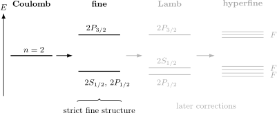
Schematic $n=2$ hierarchy, not to scale. The Lamb column isolates the radiative and associated separation of the Dirac-degenerate $2S_{1/2}$ and $2P_{1/2}$ pair. The same figure appears on the canonical fine-structure page so the boundary between the two correction layers stays explicit.

Why Coulomb Models Miss It

The nonrelativistic hydrogen Hamiltonian

$$H_{\mathrm C} = \frac{\mathbf p^2}{2m_r} - \frac{Z\alpha\hbar c}{r}$$

contains a particle moving in a static Coulomb potential. It has no dynamical electromagnetic field and no photon degrees of freedom. Solving this Hamiltonian exactly therefore cannot generate emission and reabsorption of virtual photons, polarization of the electromagnetic vacuum, or renormalization of the electron’s electromagnetic parameters.

The Dirac equation improves the one-particle description by incorporating special relativity and spin. For a point nucleus in a static Coulomb field, its energy depends on $n$ and $j$ but retains an accidental degeneracy between states with the same $n$ and $j$ and opposite values of the Dirac angular quantum number. Thus $2S_{1/2}$ and $2P_{1/2}$ remain degenerate even though they have different parity and orbital structure.

This does not mean the Dirac equation is incorrect. It means the external-field Dirac Hamiltonian omits physical interactions needed at finer resolution. The observed atom is not a bare electron in a prescribed classical field. It is a bound state of charged matter dressed by quantum electromagnetic fluctuations, with a nucleus of finite mass and finite spatial structure.

Better numerics do not add missing physics

Numerical precision and model completeness are different. Diagonalizing the Schrödinger or Dirac–Coulomb Hamiltonian to more digits only approaches the spectrum of that Hamiltonian more accurately. It cannot create operators that were not included.

The right response to a systematic discrepancy is therefore a model audit:

• Which dynamical degrees of freedom are absent?
• Which parameters are bare, renormalized, or experimentally defined?
• Which reference energy has been subtracted?
• Which recoil and nuclear effects have already been absorbed into the baseline?
• At what order in $\alpha$, $Z\alpha$, and $m_e/M$ is the calculation controlled?

The Lamb shift became historically important because all five questions had to be answered together.

Size and Power Counting

For a light hydrogenic ion, several small parameters organize the calculation:

$$\begin{gathered} \alpha\ll1, \qquad Z\alpha\ll1, \\ \frac{m_e}{M}\ll1, \qquad \frac{r_N}{a_0/Z}\ll1. \end{gathered}$$

Here $M$ and $r_N$ are the nuclear mass and characteristic charge radius. The scales are parametrically

$$\begin{aligned} E_{\mathrm{gross}} &\sim m_ec^2(Z\alpha)^2, \\ E_{\mathrm{fine}} &\sim m_ec^2(Z\alpha)^4, \\ E_{\mathrm{rad}} &\sim \frac{\alpha}{\pi} m_ec^2(Z\alpha)^4 \\ &\quad\times \left(\text{logs and coefficients}\right). \end{aligned}$$

For hydrogen, the radiative scale is often summarized as order $\alpha^5m_ec^2$. The logarithm $\ln[(Z\alpha)^{-2}]$ and state-dependent coefficients are numerically important, so power counting predicts the neighborhood, not the measured frequency.

A correction ledger

A precision level calculation can be organized schematically as

$$\begin{aligned} E_a &= E_a^{\mathrm{DC}}(m_r) +\Delta E_a^{\mathrm{SE}} \\ &\quad +\Delta E_a^{\mathrm{VP}} +\Delta E_a^{\mathrm{rec}} \\ &\quad +\Delta E_a^{\mathrm{rad-rec}} +\Delta E_a^{\mathrm{nuc}} +\cdots . \end{aligned}$$

The labels denote a reduced-mass Dirac–Coulomb reference, electron self-energy, vacuum polarization, recoil, radiative-recoil, and nuclear-structure contributions. Higher-loop radiative terms, anomalous-moment effects, and other small corrections are contained in a more detailed ledger.

For the classic interval, each symbol means a difference:

$$\Delta E_{\mathrm L}^{(2)} = \sum_X \left[ \Delta E_{2S_{1/2}}^X - \Delta E_{2P_{1/2}}^X \right].$$

The decomposition is useful only when every term uses compatible masses, nuclear conventions, regulators, and perturbative orders. Adding numbers copied from unrelated schemes can double count recoil or omit a matching term.

Contribution	Physical content	Role in electronic hydrogen
electron self-energy	bound electron emits and reabsorbs virtual photons	dominant positive contribution to the classic interval
vacuum polarization	charged virtual pairs modify photon propagation and the short-range Coulomb potential	smaller contribution, opposite in sign to the dominant interval shift
recoil	the proton is dynamical, not an infinitely heavy source	mass-ratio correction beyond simple reduced mass
radiative recoil	radiative and recoil expansions interact	required in precision comparisons
finite charge radius	the proton’s charge is spatially distributed	shifts $S$ states most strongly
nuclear polarizability	the proton can be virtually excited	tiny in electronic hydrogen, much more consequential in muonic systems

Electron Self-Energy

In QED, a charged particle interacts with the electromagnetic field it sources. Perturbatively, the electron can emit and reabsorb a virtual photon before returning to the observed state. For a free electron, this self-interaction contributes to the relation between bare and measured mass. For a bound electron, the Coulomb field changes the available intermediate states and energy denominators, leaving a state-dependent remainder after the free-particle mass contribution is renormalized.

That remainder is the dominant source of the positive hydrogen $2S_{1/2}$–$2P_{1/2}$ separation. It is not an arbitrary extra potential. It is extracted from the pole or energy eigenvalue of the interacting bound system after a consistent renormalization prescription has fixed the physical electron mass and charge.

Leading low-Z structure

For a point nucleus of infinite mass, the one-loop self-energy of a low-$Z$ hydrogenic $nS$ level has the schematic expansion

$$\begin{aligned} \Delta E_{nS}^{\mathrm{SE}} &= \frac{\alpha}{\pi} \frac{(Z\alpha)^4}{n^3} m_ec^2 \\ &\quad\times \Bigg[ \frac43 \ln\frac{1}{(Z\alpha)^2} +\frac{10}{9} \\ &\qquad -\frac43\ln k_0(nS) +\cdots \Bigg]. \end{aligned}$$

The quantity $\ln k_0(nS)$ is the Bethe logarithm. It summarizes a weighted contribution from the full spectrum of virtual atomic excitations. Despite its name, it is a state-dependent dimensionless number, not merely the logarithm of a single classical frequency.

This expression is useful for scale and structure. It is not a stand-alone precision prediction for the $2S_{1/2}$–$2P_{1/2}$ interval because:

• the $2P_{1/2}$ state also has a self-energy shift;
• recoil and reduced-mass factors have been idealized;
• vacuum polarization and nuclear structure are absent;
• higher powers of $Z\alpha$ and higher loops matter at sufficient precision;
• the low-$Z$ expansion is not the best organization for all ions.

Why S states are especially sensitive

Hydrogenic $S$ states have nonzero probability density at the origin,

$$|\psi_{nS}(0)|^2 = \frac{Z^3}{\pi n^3a_\mu^3}, \qquad a_\mu = \frac{\hbar}{m_rc\alpha}.$$

Many short-distance operators therefore act strongly on $S$ states. This observation helps explain the hierarchy but should not be promoted into a complete derivation. Self-energy samples a range of photon energies and intermediate bound and continuum states; it is not determined solely by $|\psi(0)|^2$. States with $\ell>0$ also receive radiative shifts.

Vacuum Polarization

The Coulomb interaction is mediated by the electromagnetic field. In QED, a virtual photon can fluctuate into a charged particle–antiparticle pair and back. This modifies the photon propagator and hence the effective electrostatic interaction. The leading electron-loop correction to the Coulomb potential is called the Uehling potential.

For a point nucleus it is short ranged on the electron Compton scale $\hbar/(m_ec)$. Schematically,

$$\begin{aligned} \delta V_{\mathrm U}(r) &= -\frac{Z\alpha\hbar c}{r} \frac{2\alpha}{3\pi} \\ &\quad\times \int_1^\infty dt\, e^{-2m_ecrt/\hbar} \\ &\qquad\times \left(1+\frac{1}{2t^2}\right) \frac{\sqrt{t^2-1}}{t^2}. \end{aligned}$$

The correction is most important for wavefunctions that penetrate the nuclear region. In electronic hydrogen, vacuum polarization makes the short-distance potential slightly more attractive and lowers the $2S$ level relative to what self-energy alone would predict. It therefore reduces the positive interval defined on this page.

At leading order in a low-$Z$ contact expansion, an $nS$ shift scales as

$$\Delta E_{nS}^{\mathrm{VP}} \sim -\frac{4\alpha}{15\pi} \frac{(Z\alpha)^4}{n^3} m_ec^2.$$

The absence of the large self-energy logarithm helps explain why this contribution is smaller for ordinary hydrogen. In muonic atoms, the orbital radius is much closer to the electron Compton and nuclear scales, and electron vacuum polarization becomes a leading part of the measured Lamb interval.

What “Vacuum Fluctuations” Does and Does Not Explain

It is common to say that vacuum fluctuations make the electron jitter, smearing the Coulomb potential and shifting $S$ levels. This can provide intuition for the sign and short-distance sensitivity of part of the effect. It is not a complete or unique explanation.

Several cautions matter:

• A physical level interval is gauge independent, but an informal split into “electron position fluctuations” and “field fluctuations” need not be.
• Self-energy, vacuum polarization, vertex terms, recoil, and matching contributions must be assembled according to a controlled expansion.
• The vacuum is not a classical random electromagnetic medium with a directly observable field trajectory.
• A virtual particle is an internal element of a perturbative calculation, not a short-lived on-shell object that can be detected between emission and absorption.
• Renormalization is not the act of discarding an arbitrary infinity; it fixes theory parameters through physical conditions and leaves finite predictions for observables.

A better conceptual statement is: the interacting electron–nucleus–electromagnetic-field system has bound-state energies different from those of an electron in a prescribed static Coulomb field. QED calculates those differences systematically.

Bethe’s 1947 Calculation

Lamb and Retherford announced the unexpected $2S_{1/2}$–$2P_{1/2}$ separation in 1947. Soon afterward, Hans Bethe showed that the dominant shift could be estimated using nonrelativistic radiation theory if the free-electron self-energy already contained in the measured electron mass was subtracted.

The logic was more important than any one numerical approximation:

1. Compute the radiative energy correction for a bound electron.
2. Identify the corresponding free-electron contribution.
3. Express the result in terms of the observed electron mass rather than an unobservable bare mass.
4. Retain the finite difference that depends on the atomic state.
5. Use the relativistic electron scale to delimit a nonrelativistic calculation whose ultraviolet completion was not yet fully built into the method.

Bethe obtained about $1040\ \mathrm{MHz}$ for the dominant hydrogen shift, strikingly close to the observed scale. The calculation did not constitute the final relativistic theory: its cutoff treatment, omitted vacuum-polarization and relativistic pieces, and approximate Bethe logarithm were subsequently improved. Its achievement was to demonstrate that the discrepancy had the right size and sign once electromagnetic self-energy was connected to a physical mass-renormalization condition.

Modern bound-state QED replaces the historical cutoff argument with systematic renormalized calculations or effective-field-theory matching. Bethe’s subtraction nevertheless remains an excellent conceptual doorway: a measured mass already includes free-space electromagnetic dressing, so the atomic observable is a change in dressing caused by binding, not the total electromagnetic self-energy of a point charge.

The Lamb–Retherford Experiment

The original experiment exploited a fortunate lifetime contrast. Hydrogen’s $2S$ state is metastable because a one-photon electric-dipole transition to $1S$ is forbidden in the leading approximation. The $2P$ state decays rapidly to $1S$ through an allowed electric-dipole transition.

The experimental sequence was, schematically:

1. Prepare a beam containing metastable $2S$ hydrogen atoms.
2. Send the beam through a radio-frequency or microwave interaction region.
3. Tune the field to drive transitions from $2S$ into a nearby $2P$ level.
4. Let the short-lived $2P$ population decay before reaching the metastable detector.
5. Observe a loss of metastable signal as the applied frequency crosses resonance.

The resonance frequency revealed that $2S_{1/2}$ and $2P_{1/2}$ were not degenerate. Microwave technology developed during the Second World War made a level separation near $1\ \mathrm{GHz}$ experimentally accessible.

Why the measurement is not “seeing vacuum particles”

The detector observes atoms, photons, or a loss of metastable population. The Lamb shift is inferred from a resonance condition after accounting for fields, line shapes, hyperfine components, motion, and apparatus response. The experiment tests the energy spectrum of the complete interacting system; it does not image a virtual photon or electron–positron pair.

Precision measurement ledger

A modern interval determination must specify at least:

• which hyperfine components or centroid define each level;
• electric and magnetic fields, including motional Stark effects;
• Doppler, recoil, transit-time, and line-shape corrections;
• microwave phase, power, polarization, and spatial inhomogeneity;
• state preparation and quenching efficiencies;
• correlations among fitted frequencies and systematic corrections;
• the theoretical convention used to extract a proton radius or QED remainder.

The reported frequency is an experimental observable. The labels “self-energy contribution” and “proton-size contribution” arise only after theoretical decomposition.

Why the Lamb Shift Matters Experimentally

A precision test of bound-state QED

Hydrogen is simple enough that radiative, recoil, and nuclear effects can be calculated in a controlled hierarchy, yet rich enough to test their interplay. Agreement across $1S$, $2S$, $2P$, and higher levels probes more than a single fitted constant because different states weight short-distance, recoil, and logarithmic terms differently.

The classic interval was historically decisive, but modern tests use networks of transition frequencies. An optical transition generally contains the Rydberg scale plus differences of Lamb shifts:

$$\begin{aligned} h\nu_{a\to b} &= E_b-E_a, \\ &= h cR_\infty \left(\mathcal R_b-\mathcal R_a\right) \\ &\quad +L_b-L_a +\cdots . \end{aligned}$$

Here $\mathcal R_a$ denotes the dimensionless leading Coulomb factor for level $a$. Several frequencies are needed to separate $R_\infty$, nuclear size, and radiative contributions without hidden degeneracies in the fit.

Sensitivity to the proton charge radius

A finite nuclear charge distribution softens the Coulomb potential at very small radius. For a hydrogenic $nS$ state, the leading finite-size correction scales as

$$\Delta E_{nS}^{\mathrm{size}} \simeq \frac{2}{3} \frac{(Z\alpha)^4}{n^3} m_rc^2 \left( \frac{m_rcr_p}{\hbar} \right)^2,$$

where $r_p$ is the proton root-mean-square charge radius in hydrogen. The correction is proportional to $m_r^3r_p^2$ when written in natural units. It is therefore much larger in muonic hydrogen, whose reduced mass is roughly $186$ times the electronic-hydrogen reduced mass.

This sensitivity made muonic-hydrogen Lamb spectroscopy a powerful proton-radius probe. It also created the historical “proton-radius puzzle” when early muonic extractions disagreed with then-standard electronic and scattering determinations. Later electronic-hydrogen measurements, including a direct $n=2$ Lamb-shift determination reported in 2019, favored a smaller radius compatible with the muonic scale within their uncertainties. Precision work continues to test consistency among spectroscopy, scattering, QED calculations, and nuclear-structure inputs.

The extracted radius is model dependent in a controlled sense: it is a parameter in an electromagnetic form-factor expansion combined with calculated radiative, recoil, and polarizability terms. It is not a photograph of a hard spherical boundary.

Determining constants requires a correlated fit

Hydrogen frequencies constrain both the Rydberg constant and the proton radius. Changing $R_\infty$ shifts the gross spectrum, while changing $r_p$ primarily shifts states with density near the origin. A single transition often cannot determine both independently. CODATA adjustments therefore combine multiple measurements and theoretical expressions, retain correlations, and enlarge uncertainties when the input data are statistically inconsistent.

How the Lamb Shift Leads to QED

The Lamb shift forces a transition from one-particle quantum mechanics to quantum field theory because the missing degrees of freedom are field quanta. A complete formulation requires:

• a quantized Dirac field for electrons and positrons;
• a quantized electromagnetic gauge field;
• the QED interaction between current and gauge potential;
• regularization and renormalization conditions;
• bound-state methods that locate energy poles rather than only free-particle scattering amplitudes;
• matching across the hard electron scale, atomic momentum scale, and binding-energy scale.

The same physics can be organized in several compatible frameworks. Covariant bound-state QED keeps relativistic propagators and loop corrections explicit. Nonrelativistic QED integrates out hard modes and represents them through Wilson coefficients multiplying local and nonlocal operators. Either route must reproduce the same observable interval when carried to the same order with consistent inputs.

Continue on QFT.org

The live QFT.org hub and its graduate guide provide the field-theory continuation. The relevant route is:

1. quantum electrodynamics and gauge invariance;
2. regularization, renormalization, and physical parameter definitions;
3. electron self-energy and the renormalized fermion propagator;
4. vacuum polarization and the dressed photon propagator;
5. effective-field-theory matching for bound states.

As of this page’s review date, those subjects are visible in the public QFT.org architecture but do not all have stable deep article routes. The links above therefore point to the live hub and guide rather than inventing dead destinations.

What This Page Does Not Derive

This overview deliberately stops before:

• evaluating a covariant one-loop electron self-energy diagram in a Coulomb field;
• proving the Ward–Takahashi identity or charge-renormalization relations;
• deriving the Uehling potential from the photon polarization tensor;
• separating high- and low-energy contributions in nonrelativistic QED;
• calculating Bethe logarithms numerically;
• deriving two-loop, three-loop, radiative-recoil, or nuclear-polarizability terms;
• treating high-$Z$ ions nonperturbatively in $Z\alpha$;
• reproducing a modern proton-radius or CODATA least-squares adjustment.

Those are substantial calculations with their own regulators, conventions, and uncertainty budgets. The purpose here is to make their physical roles and interfaces unambiguous.

Common Mistakes

• Calling the whole $2P_{3/2}$–$2P_{1/2}$ splitting the Lamb shift. That interval is led by fine structure; the classic Lamb interval compares $2S_{1/2}$ with $2P_{1/2}$.
• Saying Schrödinger theory predicts the wrong Lamb shift. The static Schrödinger Hamiltonian does not contain the field degrees of freedom required to predict it.
• Treating the Dirac equation as refuted. The ideal external-field model is an incomplete baseline, not a failed relativistic equation.
• Equating the Lamb shift with self-energy alone. Self-energy dominates ordinary hydrogen’s classic interval, but vacuum polarization, recoil, radiative recoil, and nuclear structure matter.
• Describing virtual particles as directly observed transient objects. They are internal elements of a perturbative representation; the observed quantity is the level interval.
• Using $|\psi(0)|^2$ as the entire explanation. Contact sensitivity is important, but radiative shifts also involve a spectrum of intermediate states and multiple momentum scales.
• Quoting $1057.845\ \mathrm{MHz}$ without naming the interval. State ordering, hyperfine centroid, isotope, and correction convention must be stated.
• Adding published contributions with incompatible baselines. Reduced mass, recoil, proton size, and renormalized parameters can otherwise be counted twice.
• Calling renormalization arbitrary subtraction. Renormalization conditions tie parameters to measured quantities and make predictions for other observables.
• Treating a spectroscopic proton radius as a hard geometric edge. It is an electromagnetic form-factor moment inferred within a complete theory model.

Exercises

1. Track the surviving degeneracy

State the degeneracy pattern of $2S_{1/2}$, $2P_{1/2}$, and $2P_{3/2}$ in (a) the spin-independent Schrödinger Coulomb model, (b) the ideal point-nucleus Dirac–Coulomb model, and (c) the model after the Lamb correction is included but hyperfine structure is omitted.

Solution

In the spin-independent Schrödinger Coulomb model, the energy depends only on $n$. All three labels belong to the same $n=2$ energy once spin is attached as a passive degeneracy.

In the ideal Dirac–Coulomb model, the energy depends on $n$ and $j$. The $2P_{3/2}$ level separates from the two $j=1/2$ levels, while

$$E_{2S_{1/2}}^{\mathrm D} = E_{2P_{1/2}}^{\mathrm D}.$$

After radiative and associated Lamb corrections are included, the $2S_{1/2}$ and $2P_{1/2}$ degeneracy is lifted. For ordinary hydrogen the $2S_{1/2}$ level is higher. Hyperfine structure would subsequently split each electronic level according to nuclear spin, but it is excluded here.

2. Estimate the radiative frequency scale

Use

$$\Delta E_{2S}^{\mathrm{lead}} \sim \frac{\alpha}{\pi} \frac{\alpha^4}{8} m_ec^2 \frac43\ln\frac{1}{\alpha^2}$$

with $\alpha^{-1}=137.0$ and $m_ec^2/h=1.236\times10^{20}\ \mathrm{Hz}$. Estimate the frequency and explain why agreement only at the order-of-magnitude level is expected.

Solution

The dimensionless logarithm is

$$\ln\frac{1}{\alpha^2} \simeq 2\ln 137 \simeq 9.84.$$

The prefactor before the logarithmic coefficient is approximately

$$\frac{\alpha^5}{8\pi} \frac{m_ec^2}{h} \simeq 1.0\times10^8\ \mathrm{Hz}.$$

Multiplying by $4(9.84)/3\simeq13.1$ gives

$$\frac{\Delta E_{2S}^{\mathrm{lead}}}{h} \sim 1.3\times10^9\ \mathrm{Hz}.$$

This is in the gigahertz neighborhood of the observed interval. The estimate omits the Bethe logarithm, constant and higher-order self-energy terms, the $2P_{1/2}$ shift, vacuum polarization, recoil, and nuclear structure. Its job is scale prediction, not precision agreement.

3. Test a contact perturbation

Suppose a short-distance correction is approximated by

$$\delta V(\mathbf r) = C\delta^3(\mathbf r).$$

Find its first-order shift for a hydrogenic state and explain the $n$ and $\ell$ dependence.

Solution

First-order perturbation theory gives

$$\Delta E_{n\ell m} = C|\psi_{n\ell m}(0)|^2.$$

Near the origin, a regular Coulomb radial wavefunction behaves as $R_{n\ell}(r)\propto r^\ell$. Therefore it vanishes at $r=0$ for every $\ell>0$. For an $S$ state,

$$\Delta E_{nS} = C\frac{Z^3}{\pi n^3a_\mu^3}.$$

Thus a contact term selects $S$ states and scales as $Z^3/n^3$ through the wavefunction density. This explains why short-range vacuum-polarization and finite-size operators distinguish $S$ from $P$ states strongly. It does not imply that every radiative correction is exactly local.

4. Explain the metastable-beam signal

Why does driving a $2S\to2P$ transition reduce the metastable-atom signal in a Lamb–Retherford-type experiment? Why is the signal loss evidence for a level interval rather than direct evidence for a particular virtual-particle picture?

Solution

The $2S$ state is metastable because its direct one-photon electric-dipole decay to $1S$ is forbidden in the leading approximation. A resonant field transfers population into $2P$, which has an allowed and rapid electric-dipole decay to $1S$. Those atoms no longer arrive at a detector designed to count metastable $2S$ atoms, so the signal decreases on resonance.

The resonance establishes an energy difference through $h\nu=E_{2S}-E_{2P}$ after apparatus corrections. Connecting that interval to self-energy, vacuum polarization, recoil, and nuclear structure requires theory. The detector does not distinguish which internal QED representation produced the energy shift.

5. Compare electronic and muonic size sensitivity

The leading finite-size shift scales approximately as $m_r^3r_p^2$ at fixed $Z$ and $n$. The reduced-mass ratio for muonic to electronic hydrogen is about $186$. Estimate the enhancement of finite-size sensitivity in muonic hydrogen.

Solution

At fixed proton radius,

$$\frac{\Delta E_{\mathrm{size}}^{\mu\mathrm H}} {\Delta E_{\mathrm{size}}^{\mathrm H}} \sim \left( \frac{m_r^{\mu\mathrm H}} {m_r^{\mathrm H}} \right)^3 \simeq 186^3.$$

Numerically,

$$186^3 \simeq 6.4\times10^6.$$

This millionfold enhancement explains why muonic-hydrogen spectroscopy is exceptionally sensitive to proton size. A complete comparison still requires the much larger electron-vacuum-polarization contribution, recoil, two-photon exchange, proton polarizability, and hyperfine effects appropriate to the measured muonic transition.

Cross-Links

• Fine Structure establishes the relativistic level hierarchy and the surviving $2S_{1/2}$–$2P_{1/2}$ Dirac degeneracy.
• Hydrogen as Atomic Prototype places radiative shifts among recoil, hyperfine, nuclear-size, and external-field corrections.
• Degeneracy of the Hydrogen Atom explains the nonrelativistic Coulomb degeneracy before spin and relativity are added.
• Hydrogen Atom is the canonical home for Coulomb eigenstates and wavefunctions.
• Dirac Equation and Pauli Equation supply compact relativistic formula references.
• Atomic Spectra Experiment Entry gives the broader spectroscopy and calibration context.
• AMO Experiment Index separates the Lamb–Retherford detector record from the QED inference and compares it with other landmark AMO experiments.
• Precision Spectroscopy develops the correction, covariance, constants, and anomaly-inference framework needed to turn a measured interval into a precision test.
• Bridge to QFT Roadmap prepares the conceptual move from quantum-mechanical systems to quantized fields.

References

1. W. E. Lamb, Jr. and R. C. Retherford, “Fine Structure of the Hydrogen Atom by a Microwave Method,” Physical Review 72, 241–243 (1947), doi:10.1103/PhysRev.72.241.
2. H. A. Bethe, “The Electromagnetic Shift of Energy Levels,” Physical Review 72, 339–341 (1947), doi:10.1103/PhysRev.72.339.
3. S. R. Lundeen and F. M. Pipkin, “Measurement of the Lamb Shift in Hydrogen, $n=2$,” Physical Review Letters 46, 232–235 (1981), doi:10.1103/PhysRevLett.46.232.
4. A. E. Kramida, “A Critical Compilation of Experimental Data on Spectral Lines and Energy Levels of Hydrogen, Deuterium, and Tritium,” Atomic Data and Nuclear Data Tables 96, 586–644 (2010), with erratum 126, 295–298 (2019), doi:10.1016/j.adt.2010.05.001.
5. M. I. Eides, H. Grotch, and V. A. Shelyuto, “Theory of Light Hydrogenlike Atoms,” Physics Reports 342, 63–261 (2001), doi:10.1016/S0370-1573(00)00077-6.
6. V. A. Yerokhin, K. Pachucki, and V. Patkóš, “Theory of the Lamb Shift in Hydrogen and Light Hydrogen-Like Ions,” Annalen der Physik 531, 1800324 (2019), doi:10.1002/andp.201800324.
7. P. J. Mohr, D. B. Newell, B. N. Taylor, and E. Tiesinga, “CODATA Recommended Values of the Fundamental Physical Constants: 2022,” Reviews of Modern Physics 97, 025002 (2025), doi:10.1103/RevModPhys.97.025002.
8. N. Bezginov et al., “A Measurement of the Atomic Hydrogen Lamb Shift and the Proton Charge Radius,” Science 365, 1007–1012 (2019), doi:10.1126/science.aau7807.
9. A. Antognini et al., “Proton Structure from the Measurement of $2S$–$2P$ Transition Frequencies of Muonic Hydrogen,” Science 339, 417–420 (2013), doi:10.1126/science.1230016.
10. R. G. Bullis et al., “Precision Spectroscopy of $2S$–$nS$ Transitions in Atomic Hydrogen: A Determination of the Proton Charge Radius,” Physical Review Letters 136, 123001 (2026), doi:10.1103/lgl2-6cb8.
11. H. A. Bethe and E. E. Salpeter, Quantum Mechanics of One- and Two-Electron Atoms (Springer, 1957), Chapters 4–6.
12. U. D. Jentschura, Quantum Electrodynamic Bound-State Calculations and Large-Order Perturbation Theory (Springer, 2004), doi:10.1007/b99673.