Hydrogen as Atomic Prototype

Hydrogen is the prototype that connects an exactly solvable quantum Hamiltonian to an experimentally resolved atom. Its Coulomb solution supplies shells, orbitals, degeneracies, and a spectral-series law. Successively finer measurements then reveal reduced-mass effects, relativistic structure, the Lamb shift, hyperfine structure, nuclear size, and external-field shifts.

This page interprets that hierarchy for atomic physics. It does not rederive the Coulomb spectrum or normalized wavefunctions: those belong to Hydrogen Atom, Radial Wavefunctions, and Atomic Orbitals. The goal here is to understand what hydrogen teaches, which idealizations each label assumes, and why real spectral lines contain more structure than $E_n\propto-1/n^2$.

Why Hydrogen Is the Prototype

Hydrogen is not merely the simplest atom. It is unusually useful because several theoretical and experimental advantages coincide:

• the internal nonrelativistic problem reduces exactly to one relative coordinate;
• the central Coulomb potential makes angular momentum and parity explicit;
• the bound and continuum spectra can be described analytically;
• the absence of electron–electron interaction isolates recoil, relativistic, radiative, and nuclear effects;
• transition frequencies can be measured at resolutions far beyond the gross binding scale;
• hydrogenic scaling extends the model to one-electron ions;
• deviations from the ideal spectrum identify which additional interaction is being resolved.

Hydrogen teaches cleanly	Hydrogen does not teach by itself
central-potential quantum numbers	electron screening and shell filling
radial and angular wavefunction structure	exchange and electron correlation
bound-state accumulation at an ionization threshold	multi-electron term systems and configuration mixing
degeneracy from rotations and hidden Coulomb symmetry	bonding and nuclear motion in molecules
transition-frequency series	many-body collective behavior
a controlled hierarchy of small corrections	arbitrary high-$Z$ relativistic structure

Hydrogen is therefore a reference problem against which more complicated models are organized. It should not be stretched into a claim that every atom is “hydrogen with corrections.”

Model Layers

After separating center-of-mass motion, the leading relative-coordinate Hamiltonian is

$$H_{\mathrm C} =\frac{\mathbf p^2}{2\mu} -\frac{e^2}{4\pi\epsilon_0r},$$

where

$$\mu=\frac{m_em_p}{m_e+m_p}$$

is the electron–proton reduced mass. The zero of energy is conventionally the separated electron and proton at rest, so bound levels have negative energy and the continuum begins at $E=0$.

A real-hydrogen level may be organized schematically as

$$\begin{aligned} E={}&E_{\mathrm C} +\Delta E_{\mathrm{fs}}\\ &+\Delta E_{\mathrm{recoil}} +\Delta E_{\mathrm{QED}}\\ &+\Delta E_{\mathrm{hfs}} +\Delta E_{\mathrm{nuc}} +\Delta E_{\mathrm{ext}}. \end{aligned}$$

This decomposition is an ordering device, not a set of separately observable boxes. Precision calculations define a reference Hamiltonian and combine relativistic, recoil, radiative, and nuclear effects consistently to avoid double counting.

Resolution determines the right model

Target	Minimum useful description
shell ordering and approximate ionization energy	reduced-mass Schrödinger–Coulomb model
$j$-resolved optical structure	relativistic fine structure plus recoil at the required order
$2S_{1/2}$–$2P_{1/2}$ separation	QED and nuclear corrections beyond the Dirac–Coulomb degeneracy
ground-state microwave hyperfine line	nuclear spin, magnetic moments, QED, recoil, and nuclear structure
precision $1S$–$2S$ comparison	a complete uncertainty budget for theory, fields, motion, line shape, and constants

Calling hydrogen “exactly solvable” always refers to a specified ideal Hamiltonian. It does not mean every observed hydrogen frequency has a closed-form exact expression.

Quantum Numbers and Their Meaning

The spinless Coulomb eigenfunctions may be labeled $|n\ell m_\ell\rangle$:

$$\begin{aligned} n&=1,2,3,\ldots,\\ \ell&=0,1,\ldots,n-1,\\ m_\ell&=-\ell,-\ell+1,\ldots,\ell. \end{aligned}$$

Each label answers a different question.

Label	Associated structure	Physical role
$n$	principal shell	sets the ideal Coulomb energy and radial scale
$\ell$	$L^2$ eigenvalue	sets orbital angular momentum, parity, and angular-node count
$m_\ell$	$L_z$ eigenvalue	sets projection on a chosen axis
$m_s$	$S_z$ eigenvalue	labels electron-spin projection before spin-dependent coupling
$j$	$J^2$ for $\mathbf J=\mathbf L+\mathbf S$	labels fine-structure levels in a rotationally invariant atom
$F$	$F^2$ for $\mathbf F=\mathbf I+\mathbf J$	labels hyperfine levels when nuclear and electronic angular momenta are coupled
$m_F$	$F_z$ eigenvalue	labels weak-field magnetic sublevels about a quantization axis

The orbital letter encodes $\ell$:

$$\ell=0,1,2,3,\ldots \quad\longleftrightarrow\quad s,p,d,f,\ldots .$$

Including electron spin, a real-hydrogen electronic level is often written $n{}^2L_J$. For example,

$$2{}^2P_{3/2}$$

means $n=2$, $S=1/2$, $L=1$, and $J=3/2$. The multiplicity $2S+1=2$ is not the number of magnetic substates; the $J=3/2$ level has $2J+1=4$ values of $m_J$ before hyperfine coupling and external fields are resolved.

Exact, approximate, and field-dressed labels

The full Hamiltonian decides which labels are exact. In zero field, rotational invariance preserves total angular momentum even when $L$ and $S$ are coupled. In a weak magnetic field, $F$ and $m_F$ may remain useful. In stronger fields, $F$ can mix while the projection along the field remains conserved. A database label may also denote the dominant component of a mixed state rather than an exact eigenvalue of every named operator.

The Ideal Coulomb Spectrum

The nonrelativistic bound energies are

$$E_n =-\frac{\mu c^2\alpha^2}{2n^2} =-\frac{\mu}{m_e}\frac{E_{\mathrm h}}{2n^2}.$$

This result is quoted here for interpretation; its derivation is canonical in Hydrogen Atom. Several consequences matter immediately:

1. Energy depends only on $n$ in the ideal problem.
2. Level spacing decreases as the spectrum approaches the ionization threshold.
3. The characteristic radius grows as $n^2$.
4. A fixed $n$ shell contains $n^2$ spatial states, or $2n^2$ after adding uncoupled electron spin.

The spatial count follows from

$$g_n=\sum_{\ell=0}^{n-1}(2\ell+1)=n^2.$$

Rotational symmetry explains degeneracy among the $2\ell+1$ values of $m_\ell$ at fixed $\ell$. It does not by itself explain why different $\ell$ values share an energy. That additional degeneracy is special to the Coulomb problem and is developed in Degeneracy of the Hydrogen Atom.

The n = 2 shell as a diagnostic

The ideal $n=2$ shell contains $2s$ and $2p$ orbitals at the same energy. Once spin is included:

• relativistic fine structure separates $2P_{1/2}$ and $2P_{3/2}$;
• the Dirac–Coulomb spectrum still leaves $2S_{1/2}$ and $2P_{1/2}$ degenerate at the corresponding idealized level;
• the Lamb shift lifts that remaining degeneracy;
• hyperfine interactions further split levels according to $F$;
• electric and magnetic fields split and mix magnetic sublevels.

The $n=2$ manifold is thus a compact map of the correction hierarchy.

Orbitals, Densities, and Nodes

The spatial Coulomb eigenfunctions factor as

$$\psi_{n\ell m_\ell}(r,\theta,\phi) =R_{n\ell}(r)Y_\ell^{m_\ell}(\theta,\phi).$$

The probability of finding the electron in a volume element is

$$dP=|\psi(\mathbf r)|^2d^3r.$$

After integrating over solid angle, the radial probability density is

$$\begin{aligned} P_{n\ell}(r)&=r^2|R_{n\ell}(r)|^2,\\ \int_0^\infty P_{n\ell}(r)\,dr&=1. \end{aligned}$$

The factor $r^2$ comes from the volume element. Consequently, the $1s$ wavefunction density $|\psi_{100}|^2$ is largest at the nucleus, while the probability per radial interval is maximal away from the origin. These are different statements about different densities.

For hydrogenic bound states,

$$N_{\mathrm{radial}}=n-\ell-1, \qquad N_{\mathrm{angular}}=\ell.$$

Orbital lobes are surfaces chosen to visualize amplitude, phase, or enclosed probability. They are not material boundaries and they do not trace electron trajectories. The canonical treatment of real and complex bases, nodes, and visualization conventions is Atomic Orbitals.

Spectral Series

For an ideal transition between levels $n_i>n_f$, the emitted photon satisfies

$$h\nu=E_{n_i}-E_{n_f}.$$

Using the Coulomb spectrum gives the Rydberg relation

$$\frac{1}{\lambda} =R_H\left( \frac{1}{n_f^2}-\frac{1}{n_i^2} \right),$$

where $R_H$ includes the electron–proton reduced-mass correction. The infinite-nuclear-mass constant $R_\infty$ is not numerically identical to $R_H$.

Series	Lower level $n_f$	Main spectral region
Lyman	$1$	ultraviolet
Balmer	$2$	visible and near ultraviolet
Paschen	$3$	infrared
Brackett	$4$	infrared
Pfund	$5$	infrared

Each series converges as $n_i\to\infty$. The limiting wavenumber measures the ionization energy from its lower level within the idealized model.

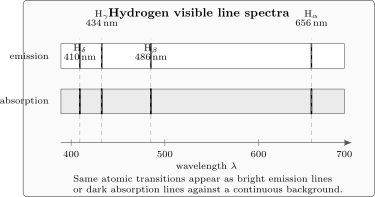
The same transition energies can appear as emission or absorption lines. This schematic is reused from the historical spectroscopy sequence; Balmer Formula owns the empirical history, while this page interprets the lines through the atomic level hierarchy.

Line position is not line intensity

The Rydberg relation predicts ideal energy differences. It does not determine whether a transition is strong. In the electric-dipole approximation, intensity depends on matrix elements such as

$$\langle f|\mathbf d\cdot\boldsymbol\epsilon|i\rangle,$$

as well as populations, polarization, observation geometry, saturation, and detection response. The leading one-electron electric-dipole rules include a parity change and $\Delta\ell=\pm1$. The Dipole Transitions page owns the angular derivation.

Ideal lines and evaluated data

Real hydrogen lines may resolve fine, Lamb, and hyperfine components or report a weighted unresolved feature. Air and vacuum wavelengths differ, and an observed line center may include Doppler, recoil, pressure, Zeeman, Stark, and instrumental shifts. For evaluated values, use the NIST Atomic Spectra Database and its linked primary sources. Its hydrogen interface distinguishes resolved fine structure from configuration-averaged data because mixing those subsets would double-count levels and lines.

What the Coulomb Model Omits

The leading Schrödinger model assumes a point electron and point nucleus interacting instantaneously through a nonrelativistic Coulomb potential. It omits:

• relativistic kinematics and spin-dependent interactions;
• radiative corrections from quantum electrodynamics;
• proton charge and magnetization distributions;
• proton spin and hyperfine coupling;
• recoil terms beyond the reduced-mass replacement;
• weak-interaction effects at much finer precision;
• external electric, magnetic, and electromagnetic fields;
• collisions, motion, blackbody radiation, and apparatus-dependent shifts;
• electron–electron repulsion, exchange, and correlation because hydrogen has only one electron.

An omitted effect is not automatically negligible. Its relevance depends on the target observable and uncertainty.

The Correction Ladder

Reduced mass and recoil

Replacing $m_e$ by $\mu$ captures the leading two-body kinematics and shifts every Coulomb energy scale. Hydrogen and deuterium therefore have different gross transition frequencies. At higher precision, recoil cannot be represented solely by a reduced mass; relativistic recoil and radiative-recoil terms enter.

Fine structure

Fine structure combines relativistic kinetic, spin–orbit, and Darwin effects in a low-energy expansion. A Dirac treatment organizes these effects relativistically. For a point Coulomb field, the Dirac energy depends on $n$ and $j$, not separately on $\ell$, which is why some opposite-parity states remain degenerate before radiative corrections. Fine Structure derives the combined leading result and its many-electron generalization.

Lamb shift

The Lamb shift denotes radiative and associated corrections that separate levels left degenerate by the ideal Dirac–Coulomb problem, most famously $2S_{1/2}$ and $2P_{1/2}$. Electron self-energy and vacuum polarization are central QED contributions, but precision theory also includes recoil and nuclear structure. A slogan about vacuum fluctuations is not a substitute for that gauge-consistent calculation. Lamb Shift Overview develops the correction ledger, experimental method, and QFT boundary.

Hyperfine structure

The proton has spin $I=1/2$ and a magnetic moment. Coupling it to electronic angular momentum gives

$$\mathbf F=\mathbf I+\mathbf J.$$

The leading magnetic-dipole model is $A\mathbf I\cdot\mathbf J$. In the $1S_{1/2}$ ground state, it separates $F=0$ and $F=1$ levels. The associated transition lies near $1.420\ \mathrm{GHz}$, corresponding to the astrophysically important 21 cm line. A precision prediction requires more than the leading contact interaction. Hyperfine Structure develops the coupling Hamiltonian, interval rule, 21 cm datum, and nuclear-structure corrections.

Finite nuclear size

S states sample the nuclear region most strongly, so their energies are especially sensitive to the proton charge distribution. Hydrogen spectroscopy, scattering measurements, and muonic-hydrogen spectroscopy constrain related nuclear parameters through different observables and theory inputs. Extracting a radius is an inference problem, not a direct picture of a hard-edged proton.

External fields

Magnetic fields produce Zeeman shifts and can change the useful coupling labels. Electric fields produce Stark shifts and mix opposite-parity states; Stark Effect in Atoms connects hydrogen’s ideal degeneracy to real-atom field scales and dynamic response. Time-dependent fields drive transitions, create AC Stark shifts, and broaden lines. A quoted “hydrogen transition frequency” is incomplete unless the field and motion conditions are controlled or extrapolated.

Added physics	New or refined labels	Representative signature
reduced mass	isotope-dependent scale	shifted Rydberg series
fine structure	$j$	splitting within an $n,\ell$ manifold
Lamb shift	retains $n,\ell,j$ labels approximately	$2S_{1/2}$–$2P_{1/2}$ separation
hyperfine interaction	$F$	microwave splitting and 21 cm line
magnetic field	$m_F$ or uncoupled projections	Zeeman components and crossings
electric field	field-dressed parity mixtures	Stark shifts and induced amplitudes
finite nuclear size	isotope and nuclear-state labels	state-dependent S-level shifts

How to Read a Hydrogen Datum

A defensible hydrogen frequency or wavelength should be accompanied by enough information to identify the physical quantity:

1. Isotope: protium, deuterium, tritium, antihydrogen, or a hydrogenic ion are different systems.
2. Initial and final levels: include $n,\ell,j,F,m_F$ to the resolution actually measured.
3. Component or centroid: state whether fine or hyperfine components are resolved, averaged, or fitted together.
4. Vacuum or medium wavelength: air wavelengths depend on a refractive-index convention.
5. Observed or Ritz value: an observed wavelength comes from a line measurement; a Ritz wavelength is inferred from optimized level energies.
6. Reference zero: level energies may be measured from the ground state or downward from the ionization limit.
7. Environmental conditions: fields, gas pressure, temperature, motion, laser intensity, and trap conditions can shift or broaden a line.
8. Uncertainty and correlations: several reported intervals may share calibration or theoretical inputs.

The NIST hydrogen handbook gives a compact evaluated entry, while the Atomic Spectra Database and its bibliography should be used for current level classifications, wavelengths, transition probabilities, and source provenance. The dedicated NIST hydrogen/deuterium calculations include relativistic, QED, recoil, and nuclear-size contributions for theoretical level values; their conventions must still be matched to the measurement being compared.

Hydrogen as a Laboratory System

Different hydrogen observables isolate different physics:

• Gross optical series test the Coulomb spectrum, reduced mass, and level assignments.
• Fine-structure intervals test relativistic and spin-dependent structure.
• The Lamb shift exposes radiative corrections beyond the Dirac–Coulomb model.
• Hyperfine transitions test magnetic moments, spin coupling, and nuclear structure.
• The $1S$–$2S$ interval combines a very narrow two-photon transition with stringent line-shape and systematic control.
• Rydberg states magnify size, field sensitivity, and near-threshold behavior.
• Photoionization and recombination probe the connection between discrete and continuum Coulomb states.
• Isotope comparisons separate mass-dependent and nuclear-structure contributions.

No single observable measures “the hydrogen energy” in isolation. Each measurement selects a transition, preparation, field geometry, and line-shape model.

Precision does not remove model dependence

A narrow line can be measured precisely while still requiring theoretical corrections to infer a constant or nuclear parameter. Conversely, a theory may predict an isolated-atom interval more precisely than an experiment realizes it because motional, field, collision, or probe shifts dominate the apparatus. Trustworthy comparisons state which inputs were fitted, which constants were held fixed, and which uncertainty components are correlated.

From Hydrogen to Other Atoms

Hydrogen supplies several reusable ideas, each with a controlled boundary.

Hydrogenic ions

One-electron ions preserve the Coulomb form with nuclear charge $Z$:

$$E_n\propto-\frac{Z^2}{n^2}, \qquad r_n\propto\frac{n^2}{Z}.$$

Relativistic and nuclear-size effects grow more important with $Z$. The Hydrogenic Ions page owns the rescaled exact solution.

Alkali atoms

An alkali atom has one valence electron outside a closed-shell core. Its high-$n$ spectrum is approximately hydrogenic, but core penetration, polarization, spin–orbit coupling, and hyperfine structure produce quantum defects and modified matrix elements. The useful analogy is “one active electron plus a structured core,” not “hydrogen with a different Rydberg constant.” Alkali Atoms develops this model through D lines, hyperfine manifolds, cooling, clocks, and Rydberg control.

Multi-electron atoms

For helium and beyond, electron–electron repulsion prevents exact separation into independent Coulomb orbitals. Hydrogenic orbitals remain valuable basis functions and qualitative labels, but antisymmetry, exchange, configuration mixing, and correlation determine the actual eigenstates. The Central-Field Approximation explains how screening turns this coupled problem into a controlled orbital reference and which residual interactions it leaves behind.

Molecules

Atomic orbitals become ingredients in molecular basis sets. Molecular eigenstates also involve multiple nuclei, bonding, vibration, rotation, and nonadiabatic coupling. The hydrogen atom motivates the basis language but does not derive molecular structure.

Common Mistakes

Repeating the exact solution instead of stating the model

Quoting $E_n$ without reduced mass, reference zero, and omitted interactions hides the physical approximation. Link to the canonical derivation and identify the resolution required here.

Treating n, ℓ, and m as exact for every real-hydrogen experiment

Fine, hyperfine, and external-field interactions change the commuting set. Labels can remain approximate and useful, but their status must be stated.

Calling an orbital a path or a hard-edged object

An orbital is a wavefunction. A plotted lobe is an isosurface or probability convention, and the electron is not confined inside it.

Confusing spatial density with radial probability

$|\psi(\mathbf r)|^2$ is probability per volume. $r^2|R(r)|^2$ is probability per radial interval after angular integration. Their maxima need not coincide.

Assuming every energy difference gives a strong line

Level spacing fixes a possible photon frequency. A transition amplitude, selection rules, populations, and experimental coupling determine whether the line is observable and how strong it is.

Using the infinite-mass Rydberg constant for real hydrogen without comment

$R_\infty$ and $R_H$ differ because the proton moves. Precision work also needs higher recoil, radiative, and nuclear corrections.

Treating “the Lamb shift” as one isolated number

Radiative shifts depend on the state and on the convention used to separate QED, recoil, and nuclear contributions. Name the levels whose difference is meant.

Reading database digits without reading metadata

Resolved components, configuration averages, observed wavelengths, Ritz wavelengths, and theoretical values are different data products. The uncertainty and cited source are part of the datum.

Exercises

Exercise 1: Inventory the n = 3 shell

List the allowed $\ell$ values and number of $m_\ell$ states in the ideal spinless $n=3$ shell. How many states are present after adding electron spin but no spin-dependent interaction?

Solution

For $n=3$, the allowed orbital quantum numbers are $\ell=0,1,2$:

$$\begin{array}{ccl} 3s:&\ell=0,&2\ell+1=1,\\ 3p:&\ell=1,&2\ell+1=3,\\ 3d:&\ell=2,&2\ell+1=5. \end{array}$$

The spatial count is

$$1+3+5=9=n^2.$$

Electron spin supplies two $m_s$ values for each spatial state, giving $18=2n^2$ states if spin-dependent interactions are absent. Fine structure reorganizes these states into $j$ multiplets without changing the total dimension of the shell subspace.

Exercise 2: Estimate Balmer alpha

Use the ideal reduced-mass Rydberg relation with $R_H\simeq1.09678\times10^7\ \mathrm{m}^{-1}$ to estimate the vacuum wavelength for the $n_i=3$ to $n_f=2$ transition. Why is this not a complete prediction of every observed H-alpha component?

Solution

The inverse wavelength is

$$\begin{aligned} \frac{1}{\lambda} &=R_H\left(\frac{1}{2^2}-\frac{1}{3^2}\right),\\ &=R_H\frac{5}{36}. \end{aligned}$$

Therefore

$$\lambda\simeq6.565\times10^{-7}\ \mathrm m =656.5\ \mathrm{nm}.$$

The estimate describes a gross-structure wavelength. Fine structure produces several allowed components, the Lamb and recoil corrections shift levels further, and hyperfine structure can be resolved at sufficient precision. Air and vacuum wavelength conventions also differ, while motion, pressure, fields, and the line-shape model affect an observed center.

Exercise 3: Track the n = 2 degeneracy

Starting from the ideal Schrödinger–Coulomb model, state what happens to $2S_{1/2}$, $2P_{1/2}$, and $2P_{3/2}$ when electron spin, Dirac fine structure, and then radiative corrections are added.

Solution

In the spin-independent Schrödinger model, all $n=2$ spatial states have the same energy, and electron spin merely doubles them. Organizing the states by $j$ gives $2S_{1/2}$, $2P_{1/2}$, and $2P_{3/2}$ labels without yet splitting them.

The ideal point-nucleus Dirac–Coulomb spectrum depends on $n$ and $j$. It separates $2P_{3/2}$ from the $j=1/2$ levels, but $2S_{1/2}$ and $2P_{1/2}$ remain degenerate. Radiative corrections lift that remaining degeneracy, producing the Lamb shift. Recoil, nuclear size, and hyperfine interactions add further refinements in real hydrogen.

Exercise 4: Two maxima in the ground state

For the hydrogenic ground state, $|\psi_{100}|^2\propto e^{-2r/a}$ with reduced-mass Bohr radius $a$. Where is the spatial probability density maximal, and where is the radial probability density maximal?

Solution

The spatial density decreases monotonically with $r$, so it is maximal at $r=0$. The radial density includes the spherical volume factor:

$$P(r)\propto r^2e^{-2r/a}.$$

Its derivative is

$$\frac{dP}{dr} \propto2re^{-2r/a}\left(1-\frac{r}{a}\right).$$

The nonzero maximum is therefore at $r=a$. There is no contradiction: one density is per unit volume and the other is per unit radius after integrating over all directions.

Exercise 5: Choose the minimum model

For each target below, name the minimum physics that must be added to the reduced-mass Schrödinger–Coulomb model: (a) identifying the Balmer series at moderate resolution, (b) predicting the $2S_{1/2}$–$2P_{1/2}$ separation, and (c) interpreting the ground-state 21 cm transition.

Solution

(a) Balmer series: The reduced-mass Coulomb spectrum plus transition selection rules is the minimum useful model. Apparatus broadening and populations are needed for an actual line shape or intensity.

(b) $2S_{1/2}$–$2P_{1/2}$ separation: The ideal Dirac–Coulomb model leaves these states degenerate. QED radiative corrections are essential, with recoil and nuclear-size terms included at the demanded precision.

(c) Ground-state 21 cm transition: Proton spin and magnetic moment must be included through hyperfine coupling. Precision work also needs radiative, recoil, and proton-structure corrections, plus environmental Zeeman and collisional effects for a measured line.

The answer depends on the target uncertainty. “Minimum model” means the first model capable of producing the observable, not necessarily the final precision theory.

Cross-Links

• Common Atomic Hamiltonians places the hydrogenic baseline beside recoil, fine, hyperfine, and external-field additions.

• Stark Effect in Atoms

• Atomic Physics

• Atomic Units and Scales

• Central-Field Approximation

• Alkali Atoms

• Rydberg Atoms Basics

• Fine Structure

• Lamb Shift Overview

• Hyperfine Structure

• Hydrogen Atom

• Hydrogenic Ions

• Atomic Orbitals

• Degeneracy of the Hydrogen Atom

• Coulomb Continuum States

• Hydrogen Spectrum Formula

• Hydrogen Angular Structure

• Dipole Transitions

References

1. C. J. Foot, Atomic Physics, Oxford University Press, 2005.
2. B. H. Bransden and C. J. Joachain, Physics of Atoms and Molecules, 2nd ed., Pearson, 2003.
3. H. A. Bethe and E. E. Salpeter, Quantum Mechanics of One- and Two-Electron Atoms, Springer, 1957.
4. H. Friedrich, Theoretical Atomic Physics, 4th ed., Springer, 2017.
5. A. E. Kramida, “A critical compilation of experimental data on spectral lines and energy levels of hydrogen, deuterium, and tritium,” Atomic Data and Nuclear Data Tables 96, 586–644 (2010), with erratum 126, 295–298 (2019), DOI: 10.1016/j.adt.2010.05.001.
6. A. Kramida, Yu. Ralchenko, J. Reader, and the NIST ASD Team, NIST Atomic Spectra Database, version 5.12, National Institute of Standards and Technology, 2024, DOI: 10.18434/T4W30F, accessed 2026-07-21.
7. U. D. Jentschura, S. Kotochigova, E.-O. Le Bigot, P. J. Mohr, and B. N. Taylor, NIST database of energy levels of hydrogen and deuterium, National Institute of Standards and Technology.
8. W. E. Lamb, Jr. and R. C. Retherford, “Fine structure of the hydrogen atom by a microwave method,” Physical Review 72, 241–243 (1947), DOI: 10.1103/PhysRev.72.241.
9. P. J. Mohr, D. B. Newell, B. N. Taylor, and E. Tiesinga, “CODATA recommended values of the fundamental physical constants: 2022,” Reviews of Modern Physics 97, 025002 (2025), DOI: 10.1103/RevModPhys.97.025002.