Continuum States of the Coulomb Problem: Overview

The attractive Coulomb Hamiltonian has more than the hydrogenic bound states. Its spectrum contains an infinite negative-energy ladder and a positive-energy continuum. The bound states describe an electron remaining attached to the nucleus; the continuum states describe ionized relative motion and Coulomb scattering. For the general language of point spectrum, continuum thresholds, spectral measures, and generalized eigenstates, see Discrete and Continuous Spectra.

This page is an overview. It explains where the continuum sits in the spectrum, how its states differ from normalizable orbitals, and why the long-range Coulomb tail changes the usual scattering asymptotics. Detailed scattering amplitudes and cross sections belong to Coulomb Scattering.

Spectral Split

For an attractive one-electron Coulomb problem,

$$\hat H = \frac{\hat{\mathbf p}^{\,2}}{2\mu} - \frac{\kappa_Z}{r}, \qquad \kappa_Z=\frac{Ze^2}{4\pi\epsilon_0},$$

the bound-state energies are

$$E_n = - \frac{E_Z}{n^2}, \qquad n=1,2,\ldots,$$

where

$$E_Z = \frac{\mu\kappa_Z^2}{2\hbar^2}.$$

These levels accumulate at $E=0$ from below. The threshold $E=0$ is the ionization threshold: it separates square-integrable bound states from positive-energy continuum states.

For $E\gt 0$, write

$$E = \frac{\hbar^2k^2}{2\mu}, \qquad k\gt 0.$$

The label $k$ is continuous. Instead of discrete states $\psi_{n\ell m}$, one uses generalized eigenfunctions such as $\psi_{k\ell m}$ or incoming/outgoing scattering states.

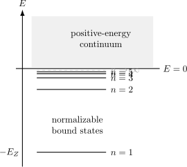
The attractive Coulomb spectrum has normalizable bound states at $E_n=-E_Z/n^2$ and a positive-energy continuum beginning at the ionization threshold $E=0$. The threshold itself is not an additional normalizable bound state.

Positive-Energy Radial Equation

For a general signed Coulomb coupling

$$V(r)=\frac{g}{r},$$

define the Coulomb parameter

$$\eta = \frac{\mu g}{\hbar^2k}.$$

Attraction has $g\lt 0$, and repulsion has $g\gt 0$. In a fixed angular-momentum channel, the reduced radial function obeys

$$\frac{d^2u_{k\ell}}{dr^2} + \left[ k^2 - \frac{2\eta k}{r} - \frac{\ell(\ell+1)}{r^2} \right] u_{k\ell} =0.$$

Near the origin, the same regularity rule as in the bound problem selects

$$u_{k\ell}(r)\sim r^{\ell+1}.$$

At large radius, however, positive-energy states do not decay. They oscillate. The continuum-state boundary condition is therefore not normalizability at infinity but an incoming, outgoing, or standing-wave convention.

Coulomb Functions

The regular positive-energy radial solutions are written in terms of Coulomb wave functions. Schematically,

$$u_{k\ell}(r) \propto F_\ell(\eta,kr),$$

where $F_\ell$ is regular at the origin. The companion function $G_\ell(\eta,kr)$ is irregular at the origin and is useful for constructing scattering combinations.

For large $\rho=kr$, the regular Coulomb function has the asymptotic form

$$F_\ell(\eta,\rho) \sim \sin \left[ \rho - \frac{\ell\pi}{2} - \eta\ln(2\rho) + \sigma_\ell \right],$$

with Coulomb phase

$$\sigma_\ell = \arg\Gamma(\ell+1+i\eta).$$

The logarithmic phase term is the warning sign that Coulomb scattering is not short-range scattering in disguise. For a short-range potential, the asymptotic radial phase is shifted by a constant phase shift. For an unscreened $1/r$ tail, the phase keeps changing logarithmically with radius.

Normalization

Bound hydrogenic states are square-normalized:

$$\int_{\mathbb R^3} \lvert\psi_{n\ell m}(\mathbf r)\rvert^2\,d^3r =1.$$

Continuum states are not square-integrable. They are generalized eigenfunctions normalized to delta functions. A common angular-momentum convention is

$$\langle \psi_{k\ell m}\vert \psi_{k'\ell' m'}\rangle = \delta(k-k') \delta_{\ell\ell'} \delta_{mm'}.$$

Different books use energy normalization or momentum-vector normalization instead. The physics is unchanged, but factors of $k$, $\mu$, and $\hbar$ move between the wavefunction and the delta function. This is why Normalization Conventions should be fixed before comparing continuum formulas.

A schematic spectral resolution has both discrete and continuous pieces:

$$\hat I = \sum_{n\ell m} \lvert\psi_{n\ell m}\rangle \langle\psi_{n\ell m}\rvert + \sum_{\ell m} \int_0^\infty dk\, \lvert\psi_{k\ell m}\rangle \langle\psi_{k\ell m}\rvert.$$

This formula suppresses normalization-convention factors, but it captures the essential point: a complete Coulomb basis requires the continuum as well as the bound ladder.

Attractive and Repulsive Cases

The attractive Coulomb potential has both bound states and continuum states. The repulsive Coulomb potential has only continuum states in the two-body point-charge problem. It has no hydrogenic bound-state ladder because the potential does not provide a well that can bind the relative coordinate.

Both signs have long-range scattering. The sign affects the Coulomb parameter $\eta$, the phase structure, and whether low-energy trajectories are focused or defocused. It does not remove the need for Coulomb-specific asymptotic conventions.

For hydrogen photoionization, electron-ion collisions, and recombination, the attractive continuum is essential: the final or intermediate state is not a plane wave, but an electron moving in the long-range field of the ion. Plane waves can be useful approximations only when the Coulomb distortion is negligible or has been handled separately.

Ionization Threshold and Large-n States

The large-$n$ bound states approach the continuum threshold:

$$E_n\to0^- \qquad \text{as} \qquad n\to\infty.$$

Their sizes grow as powers of $n$; for example, typical radii scale like $n^2a_Z$ at fixed low $\ell$. These weakly bound Rydberg states are discrete, normalizable states, not continuum states, but they sit arbitrarily close to the threshold.

At $E=0$, the qualitative behavior changes. The state is no longer a normalizable member of the bound ladder. Threshold behavior is delicate in Coulomb problems because the range is infinite, so ordinary short-range threshold formulas cannot be imported unchanged.

What This Page Does Not Derive

This overview does not derive the Rutherford cross section, exact Coulomb scattering amplitude, optical-theorem subtleties, or screened-Coulomb limits. Those belong in scattering theory.

The division of labor is:

• this page: where the continuum belongs in the Coulomb spectrum;
• Radial Schrödinger Equation: the half-line radial equation and boundary conventions;
• Coulomb Scattering: scattering amplitudes, Rutherford behavior, and long-range phase conventions;
• Partial-Wave Expansion: the central-potential scattering decomposition for short-range problems, with Coulomb caveats;
• Bound States and Scattering Poles: the broader analytic relation between spectra and scattering amplitudes.

Common Mistakes

• Treating the hydrogenic bound-state list as the whole spectrum.
• Calling positive-energy Coulomb states orbitals in the same sense as normalizable bound states.
• Normalizing continuum states to $1$ instead of to a delta function.
• Replacing Coulomb continuum states by plane waves without checking whether the long-range tail matters.
• Treating $E=0$ as an ordinary extra bound state.
• Applying short-range threshold or phase-shift formulas to an unscreened Coulomb potential without modification.
• Forgetting that repulsive Coulomb scattering has continuum states but no two-body point-Coulomb bound states.

Exercises

1. Explain why a positive-energy Coulomb eigenfunction cannot be square-normalized on all of space.

Solution

For $E\gt 0$, the radial solution oscillates at large $r$ rather than decaying exponentially. Its probability density therefore does not fall fast enough to give a finite integral over all space. Such states are generalized eigenfunctions and must be normalized to delta functions, just as free-particle momentum eigenstates are.

2. For the attractive Coulomb problem, show that the gap between adjacent high-$n$ bound levels shrinks as $n$ grows.

Solution

The bound energies are

$$E_n=-\frac{E_Z}{n^2}.$$

The adjacent spacing in magnitude is

$$E_{n+1}-E_n = -\frac{E_Z}{(n+1)^2} + \frac{E_Z}{n^2} = E_Z \left[ \frac{1}{n^2} - \frac{1}{(n+1)^2} \right].$$

For large $n$,

$$\frac{1}{n^2} - \frac{1}{(n+1)^2} \sim \frac{2}{n^3}.$$

Thus the bound levels become denser as they accumulate at $E=0$ from below.

3. In the radial equation, what changes when the Coulomb interaction is repulsive rather than attractive?

Solution

Use the signed coupling $V(r)=g/r$. Repulsion has $g\gt 0$, so

$$\eta=\frac{\mu g}{\hbar^2k}\gt 0.$$

Attraction has $g\lt 0$, so $\eta\lt 0$. The radial equation

$$u_{k\ell}'' + \left[ k^2 - \frac{2\eta k}{r} - \frac{\ell(\ell+1)}{r^2} \right]u_{k\ell} =0$$

keeps the same form, but the sign of the $1/r$ term changes through $\eta$. The attractive case can also have negative-energy bound states; the repulsive two-body point-Coulomb case cannot.

Where This Is Used

• Coulomb Potential introduces the bound-continuum split and the charge conventions used here.
• Hydrogen Atom gives the normalizable negative-energy part of the attractive Coulomb spectrum.
• Hydrogenic Ions rescales both bound and continuum Coulomb states by $Z$ and reduced mass.
• Radial Schrödinger Equation gives the radial equation whose positive-energy solutions become Coulomb functions.
• Coulomb Scattering treats the detailed long-range scattering problem.
• Normalization Conventions explains the delta-normalization choices needed for continuum states.

References

• D. J. Griffiths and D. F. Schroeter, Introduction to Quantum Mechanics, 3rd ed., Cambridge University Press, 2018.
• R. Shankar, Principles of Quantum Mechanics, 2nd ed., Springer, 1994.
• C. Cohen-Tannoudji, B. Diu, and F. Laloë, Quantum Mechanics, Wiley, 1977.
• L. D. Landau and E. M. Lifshitz, Quantum Mechanics: Non-Relativistic Theory, 3rd ed., Pergamon, 1977.
• J. R. Taylor, Scattering Theory: The Quantum Theory of Nonrelativistic Collisions, Dover, 2006.
• A. Messiah, Quantum Mechanics, Dover, 1999.